Introduction to Deep Learning and Neural Networks

Business Scenario

Welcome!

You are an AI/ML Engineer on the SmartCart AI team at NextCart Technologies. The catalog team currently uses a simple Logistic Regression model to classify products into three categories: Electronics, Grocery and Apparel

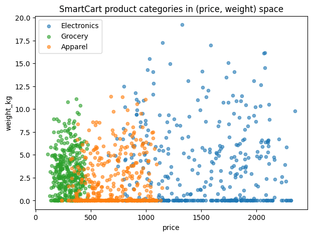
However, the model has reached a limit in its accuracy because the product attributes often overlap, making the categories difficult to separate using simple decision boundaries.

Your main task is to Build a Perceptron and a basic Artificial Neural Network (ANN) from scratch to classify SmartCart products and understand“Why was a neural network needed instead of a traditional ML model?”

Pre-Lab Preparation

Topic: Deep Learning and Neural Networks

1) What is Deep Learning, and how does it differ from traditional Machine Learning

2) The Perceptron

3) Artificial Neural Network (ANN) architecture

4) Activation functions

Git Pull

git pull origin branchName

Deep Learning vs. Traditional Machine Learning

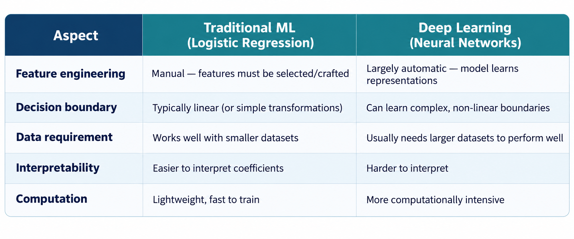
Deep Learning is a subfield of Machine Learning that uses Artificial Neural Networks with multiple layers to automatically learn patterns and representations directly from data, rather than relying on manually engineered features.

Traditional ML vs. Deep Learning

Setup

Task 1: Data Loading & Pre-processing

import numpy as np
import pandas as pd
import matplotlib.pyplot as plt
 
from sklearn.model_selection import train_test_split
from sklearn.preprocessing import StandardScaler, LabelEncoder
from sklearn.linear_model import LogisticRegression
from sklearn.metrics import accuracy_score, confusion_matrix, classification_report
 
np.random.seed(42)
plt.rcParams["figure.figsize"] = (7, 5)

Load and Inspect the SmartCart Dataset

Dataset :

DATA_PATH = "smartcart_dataset.csv"
 
df = pd.read_csv(DATA_PATH)
print("Shape:", df.shape)
print("\nMissing values per column:\n", df.isna().sum())
print("\nClass balance:\n", df["category"].value_counts())
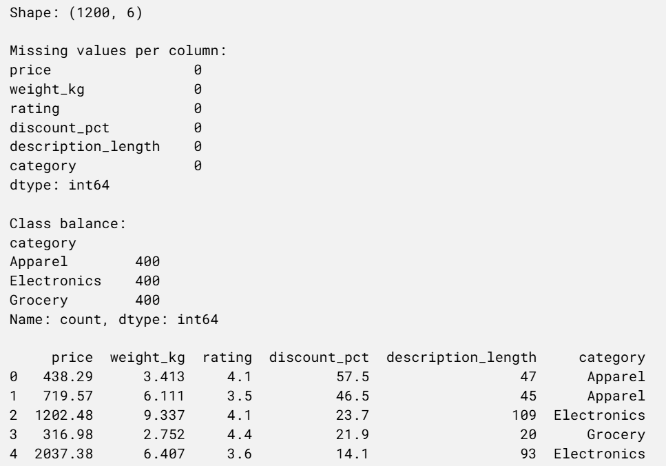
df.head()

Output

Exploratory Visualization

colors = {"Electronics": "tab:blue", "Grocery": "tab:green", "Apparel": "tab:orange"}
 
fig, ax = plt.subplots()
for cat, color in colors.items():
    subset = df[df["category"] == cat]
    ax.scatter(subset["price"], subset["weight_kg"], 
    label=cat, alpha=0.6, color=color, s=20)
ax.set_xlabel("price")
ax.set_ylabel("weight_kg")
ax.set_title("SmartCart product categories in (price, weight) space")
ax.legend()
plt.show()

Preprocessing

FEATURES = ["price", "weight_kg", "rating", "discount_pct", "description_length"]
TARGET = "category"
X = df[FEATURES].values
y_raw = df[TARGET].values
 
# Encode string labels -> integers (0, 1, 2)
label_encoder = LabelEncoder()
y = label_encoder.fit_transform(y_raw)
class_names = label_encoder.classes_
print("Classes:", dict(zip(range(len(class_names)), class_names)))
 
# Train/test split (stratified so class balance is preserved)
X_train, X_test, y_train, y_test = train_test_split(
    X, y, test_size=0.2, random_state=42, stratify=y)
 
# Standardize features (zero mean, unit variance) -- important for both models to train well
scaler = StandardScaler()
X_train_scaled = scaler.fit_transform(X_train)
X_test_scaled = scaler.transform(X_test)
 
print("Train shape:", X_train_scaled.shape, " Test shape:", X_test_scaled.shape)

Perceptron

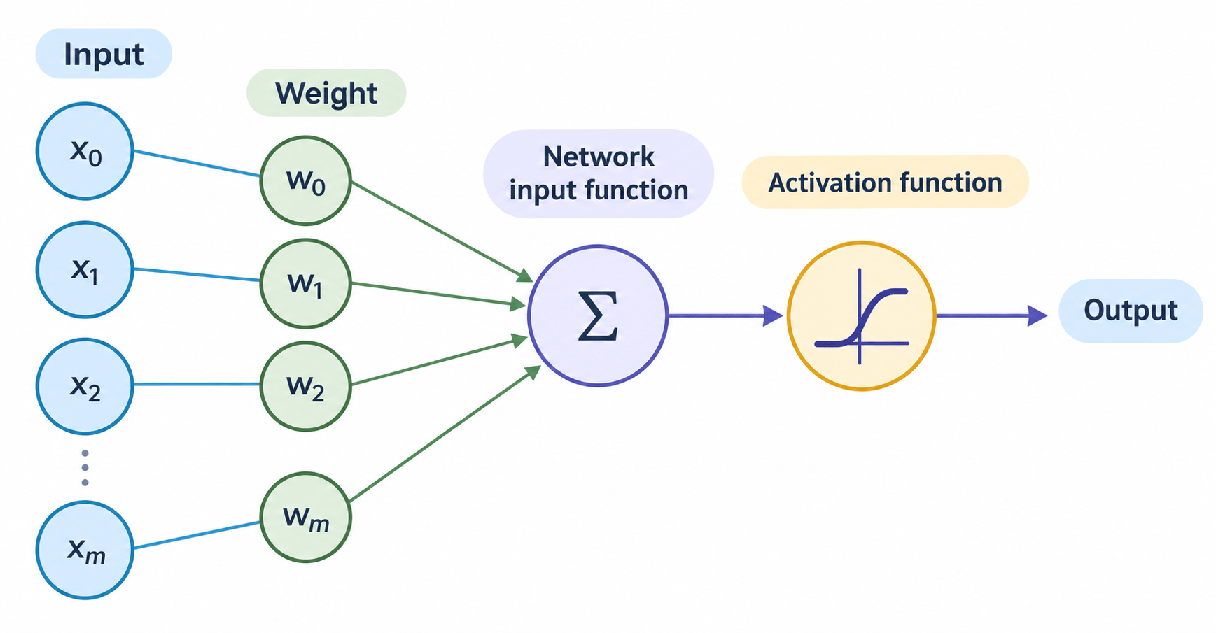
Perceptron — the simplest unit of a neural network.

It takes one or more numerical inputs, multiplies each by a weight, adds a bias and passes the result through an activation function to produce a binary output. It is the neural equivalent of a simple linear classifier.

Implement the Perceptron Class

Task 2 : Build a Perceptron From Scratch

class Perceptron:
    """Single-layer Perceptron for binary classification (+1 / -1 labels)."""
    
    def __init__(self, n_features, learning_rate=0.01, n_epochs=50):
        self.lr = learning_rate
        self.n_epochs = n_epochs
        self.weights = np.zeros(n_features)   # learnable weights
        self.bias = 0.0                       # learnable bias
    
    def net_input(self, X):
        return X @ self.weights + self.bias
    
    def predict_raw(self, X):
        return self.net_input(X)
    
    def predict(self, X):
        # step activation: +1 if the weighted sum crosses the threshold, else -1
        return np.where(self.net_input(X) >= 0, 1, -1)
    
    def fit(self, X, y):
        """y must be +1 / -1 labels. Implements the Perceptron Learning Rule."""
        for epoch in range(self.n_epochs):
            errors = 0

class Perceptron:
    """Single-layer Perceptron for binary classification (+1 / -1 labels)."""

    def __init__(self, n_features, learning_rate=0.01, n_epochs=50):
        self.lr = learning_rate
        self.n_epochs = n_epochs
        self.weights = np.zeros(n_features)   # learnable weights
        self.bias = 0.0                       # learnable bias

    def net_input(self, X):
        return X @ self.weights + self.bias

    def predict_raw(self, X):
        return self.net_input(X)

    def predict(self, X):
        # step activation: +1 if the weighted sum crosses the threshold, else -1
        return np.where(self.net_input(X) >= 0, 1, -1)

    def fit(self, X, y):
        """y must be +1 / -1 labels. Implements the Perceptron Learning Rule."""
        for epoch in range(self.n_epochs):
            errors = 0
            for xi, target in zip(X, y):
                prediction = 1 if self.net_input(xi) >= 0 else -1
                update = self.lr * (target - prediction)
                if update != 0:
                    self.weights += update * xi
                    self.bias += update
                    errors += 1
            if errors == 0:   # converged
                break
        return self

Extend to Multiclass with One-vs-Rest

class OneVsRestPerceptron:
    """Wraps K binary Perceptrons to do multiclass classification."""

    def __init__(self, n_classes, n_features, learning_rate=0.01, n_epochs=50):
        self.n_classes = n_classes
        self.models = [
            Perceptron(n_features, learning_rate, n_epochs) for _ in range(n_classes)
        ]

    def fit(self, X, y):
        for c in range(self.n_classes):
            y_binary = np.where(y == c, 1, -1)
            self.models[c].fit(X, y_binary)
        return self

class OneVsRestPerceptron:
    """Wraps K binary Perceptrons to do multiclass classification."""

    def __init__(self, n_classes, n_features, learning_rate=0.01, n_epochs=50):
        self.n_classes = n_classes
        self.models = [
            Perceptron(n_features, learning_rate, n_epochs) for _ in range(n_classes)
        ]

    def fit(self, X, y):
        for c in range(self.n_classes):
            y_binary = np.where(y == c, 1, -1)
            self.models[c].fit(X, y_binary)
        return self

    def predict(self, X):
        # score each sample against every class's Perceptron, pick the highest score
        scores = np.column_stack([m.predict_raw(X) for m in self.models])
        return np.argmax(scores, axis=1)

Train and Test the Perceptron on the SmartCart Dataset

perceptron_model = OneVsRestPerceptron(
    n_classes=len(class_names), n_features=X_train_scaled.shape[1],
    learning_rate=0.01, n_epochs=100)
perceptron_model.fit(X_train_scaled, y_train)

y_pred_perceptron = perceptron_model.predict(X_test_scaled)
perceptron_acc = accuracy_score(y_test, y_pred_perceptron)

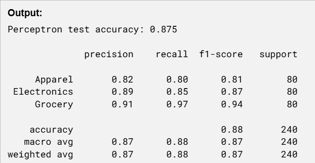
print(f"Perceptron test accuracy: {perceptron_acc:.3f}\n")
print(classification_report(y_test, y_pred_perceptron, target_names=class_names))

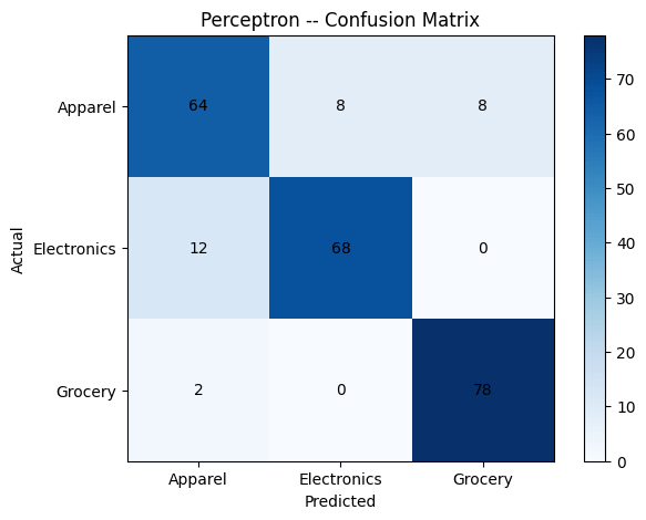
Confusion Matrix

cm_perceptron = confusion_matrix(y_test, y_pred_perceptron)

fig, ax = plt.subplots()
im = ax.imshow(cm_perceptron, cmap="Blues")
ax.set_xticks(range(len(class_names))); ax.set_xticklabels(class_names)
ax.set_yticks(range(len(class_names))); ax.set_yticklabels(class_names)
ax.set_xlabel("Predicted"); ax.set_ylabel("Actual")
ax.set_title("Perceptron -- Confusion Matrix")
for i in range(len(class_names)):
    for j in range(len(class_names)):
        ax.text(j, i, cm_perceptron[i, j], ha="center", va="center")
plt.colorbar(im)
plt.show()

Aritificial Neural Network

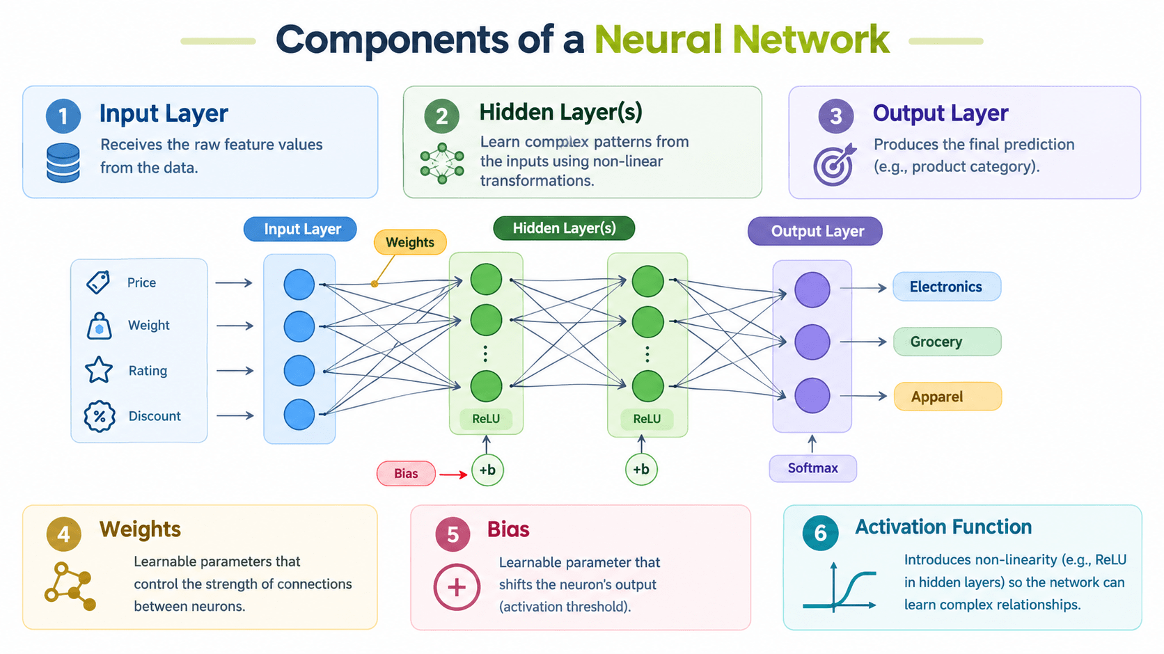
ANN Architecture — an Artificial Neural Network is built by arranging many Perceptron-like units (“neurons”) into layers, stacked so the output of one layer feeds into the next.

Define the ANN

Task 3 : Build a basic ANN and Test it on the SmartCart dataset

def one_hot(y, n_classes):
    m = np.zeros((y.shape[0], n_classes))
    m[np.arange(y.shape[0]), y] = 1
    return m


def relu(z):
    return np.maximum(0, z)


def relu_derivative(z):
    return (z > 0).astype(float)


def softmax(z):
    z_shifted = z - np.max(z, axis=1, keepdims=True)  # numerical stability
    exp_z = np.exp(z_shifted)
    return exp_z / np.sum(exp_z, axis=1, keepdims=True)


class SimpleANN:
    """Feed-forward NN: Input -> Hidden(ReLU) -> Output(Softmax). 
    Trained with plain gradient descent."""

def one_hot(y, n_classes):
    m = np.zeros((y.shape[0], n_classes))
    m[np.arange(y.shape[0]), y] = 1
    return m


def relu(z):
    return np.maximum(0, z)


def relu_derivative(z):
    return (z > 0).astype(float)


def softmax(z):
    z_shifted = z - np.max(z, axis=1, keepdims=True)  # numerical stability
    exp_z = np.exp(z_shifted)
    return exp_z / np.sum(exp_z, axis=1, keepdims=True)


class SimpleANN:
    """Feed-forward NN: Input -> Hidden(ReLU) -> Output(Softmax). 
    Trained with plain gradient descent."""

    def __init__(self, n_input, n_hidden, n_output, learning_rate=0.1, seed=42):
        rng = np.random.default_rng(seed)
        # He-style small random init
        self.W1 = rng.normal(0, np.sqrt(2.0 / n_input), (n_input, n_hidden))
        self.b1 = np.zeros((1, n_hidden))
        self.W2 = rng.normal(0, np.sqrt(2.0 / n_hidden), (n_hidden, n_output))
        self.b2 = np.zeros((1, n_output))
        self.lr = learning_rate
        self.loss_history = []

    def forward(self, X):
        self.Z1 = X @ self.W1 + self.b1
        self.A1 = relu(self.Z1)
        self.Z2 = self.A1 @ self.W2 + self.b2
        self.A2 = softmax(self.Z2)
        return self.A2

    def compute_loss(self, y_onehot, y_pred):
        eps = 1e-9  # avoid log(0)
        return -np.mean(np.sum(y_onehot * np.log(y_pred + eps), axis=1))

## Backpropagation and Training Loop

    def backward(self, X, y_onehot):
        m = X.shape[0]

        dZ2 = self.A2 - y_onehot                      # (m, n_output)
        dW2 = self.A1.T @ dZ2 / m
        db2 = np.sum(dZ2, axis=0, keepdims=True) / m

def one_hot(y, n_classes):
    m = np.zeros((y.shape[0], n_classes))
    m[np.arange(y.shape[0]), y] = 1
    return m


def relu(z):
    return np.maximum(0, z)


def relu_derivative(z):
    return (z > 0).astype(float)


def softmax(z):
    z_shifted = z - np.max(z, axis=1, keepdims=True)  # numerical stability
    exp_z = np.exp(z_shifted)
    return exp_z / np.sum(exp_z, axis=1, keepdims=True)


class SimpleANN:
    """Feed-forward NN: Input -> Hidden(ReLU) -> Output(Softmax). 
    Trained with plain gradient descent."""

    def __init__(self, n_input, n_hidden, n_output, learning_rate=0.1, seed=42):
        rng = np.random.default_rng(seed)
        # He-style small random init
        self.W1 = rng.normal(0, np.sqrt(2.0 / n_input), (n_input, n_hidden))
        self.b1 = np.zeros((1, n_hidden))
        self.W2 = rng.normal(0, np.sqrt(2.0 / n_hidden), (n_hidden, n_output))
        self.b2 = np.zeros((1, n_output))
        self.lr = learning_rate
        self.loss_history = []

    def forward(self, X):
        self.Z1 = X @ self.W1 + self.b1
        self.A1 = relu(self.Z1)
        self.Z2 = self.A1 @ self.W2 + self.b2
        self.A2 = softmax(self.Z2)
        return self.A2

    def compute_loss(self, y_onehot, y_pred):
        eps = 1e-9  # avoid log(0)
        return -np.mean(np.sum(y_onehot * np.log(y_pred + eps), axis=1))

    ## Backpropagation and Training Loop
    
    def backward(self, X, y_onehot):
        m = X.shape[0]

        dZ2 = self.A2 - y_onehot                      # (m, n_output)
        dW2 = self.A1.T @ dZ2 / m
        db2 = np.sum(dZ2, axis=0, keepdims=True) / m

        dA1 = dZ2 @ self.W2.T
        dZ1 = dA1 * relu_derivative(self.Z1)
        dW1 = X.T @ dZ1 / m
        db1 = np.sum(dZ1, axis=0, keepdims=True) / m

        self.W2 -= self.lr * dW2
        self.b2 -= self.lr * db2
        self.W1 -= self.lr * dW1
        self.b1 -= self.lr * db1

    def fit(self, X, y, n_classes, epochs=500, batch_size=32, verbose_every=50):
        y_onehot = one_hot(y, n_classes)
        n_samples = X.shape[0]

        for epoch in range(epochs):
            # shuffle each epoch
            perm = np.random.permutation(n_samples)
            X_shuffled, y_shuffled = X[perm], y_onehot[perm]

            for start in range(0, n_samples, batch_size):
                end = start + batch_size
                X_batch = X_shuffled[start:end]
                y_batch = y_shuffled[start:end]

                self.forward(X_batch)
                self.backward(X_batch, y_batch)

            # track loss on full training set once per epoch
            full_pred = self.forward(X)
            loss = self.compute_loss(y_onehot, full_pred)
            self.loss_history.append(loss)

def one_hot(y, n_classes):
    m = np.zeros((y.shape[0], n_classes))
    m[np.arange(y.shape[0]), y] = 1
    return m


def relu(z):
    return np.maximum(0, z)


def relu_derivative(z):
    return (z > 0).astype(float)


def softmax(z):
    z_shifted = z - np.max(z, axis=1, keepdims=True)  # numerical stability
    exp_z = np.exp(z_shifted)
    return exp_z / np.sum(exp_z, axis=1, keepdims=True)


class SimpleANN:
    """Feed-forward NN: Input -> Hidden(ReLU) -> Output(Softmax). 
    Trained with plain gradient descent."""

    def __init__(self, n_input, n_hidden, n_output, learning_rate=0.1, seed=42):
        rng = np.random.default_rng(seed)
        # He-style small random init
        self.W1 = rng.normal(0, np.sqrt(2.0 / n_input), (n_input, n_hidden))
        self.b1 = np.zeros((1, n_hidden))
        self.W2 = rng.normal(0, np.sqrt(2.0 / n_hidden), (n_hidden, n_output))
        self.b2 = np.zeros((1, n_output))
        self.lr = learning_rate
        self.loss_history = []

    def forward(self, X):
        self.Z1 = X @ self.W1 + self.b1
        self.A1 = relu(self.Z1)
        self.Z2 = self.A1 @ self.W2 + self.b2
        self.A2 = softmax(self.Z2)
        return self.A2

    def compute_loss(self, y_onehot, y_pred):
        eps = 1e-9  # avoid log(0)
        return -np.mean(np.sum(y_onehot * np.log(y_pred + eps), axis=1))

    ## Backpropagation and Training Loop
    
    def backward(self, X, y_onehot):
        m = X.shape[0]

        dZ2 = self.A2 - y_onehot                      # (m, n_output)
        dW2 = self.A1.T @ dZ2 / m
        db2 = np.sum(dZ2, axis=0, keepdims=True) / m

        dA1 = dZ2 @ self.W2.T
        dZ1 = dA1 * relu_derivative(self.Z1)
        dW1 = X.T @ dZ1 / m
        db1 = np.sum(dZ1, axis=0, keepdims=True) / m

        self.W2 -= self.lr * dW2
        self.b2 -= self.lr * db2
        self.W1 -= self.lr * dW1
        self.b1 -= self.lr * db1

    def fit(self, X, y, n_classes, epochs=500, batch_size=32, verbose_every=50):
        y_onehot = one_hot(y, n_classes)
        n_samples = X.shape[0]

        for epoch in range(epochs):
            # shuffle each epoch
            perm = np.random.permutation(n_samples)
            X_shuffled, y_shuffled = X[perm], y_onehot[perm]

            for start in range(0, n_samples, batch_size):
                end = start + batch_size
                X_batch = X_shuffled[start:end]
                y_batch = y_shuffled[start:end]

                self.forward(X_batch)
                self.backward(X_batch, y_batch)

            # track loss on full training set once per epoch
            full_pred = self.forward(X)
            loss = self.compute_loss(y_onehot, full_pred)
            self.loss_history.append(loss)

            if verbose_every and epoch % verbose_every == 0:
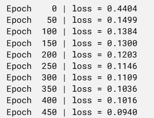
                print(f"Epoch {epoch:4d} | loss = {loss:.4f}")

        return self

    def predict(self, X):
        probs = self.forward(X)
        return np.argmax(probs, axis=1)

Train the ANN

ann_model = SimpleANN(
    n_input=X_train_scaled.shape[1],
    n_hidden=16,
    n_output=len(class_names),
    learning_rate=0.1,
    seed=42)

ann_model.fit(X_train_scaled, y_train, n_classes=len(class_names), 
epochs=500, batch_size=32, verbose_every=50)

Plot a graph

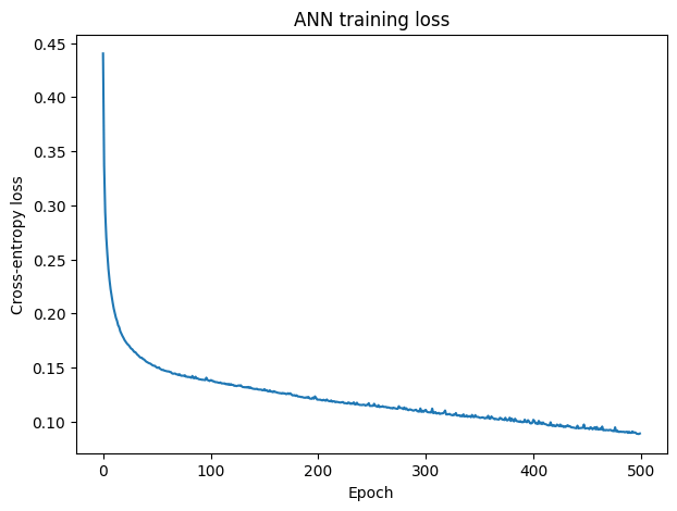
plt.plot(ann_model.loss_history)
plt.xlabel("Epoch")
plt.ylabel("Cross-entropy loss")
plt.title("ANN training loss")
plt.show()

Predict and Evaluate

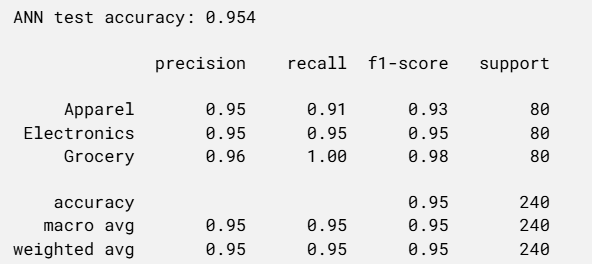
y_pred_ann = ann_model.predict(X_test_scaled)

ann_acc = accuracy_score(y_test, y_pred_ann)

print(f"ANN test accuracy: {ann_acc:.3f}\n")
print(classification_report(y_test, y_pred_ann, 
target_names=class_names))

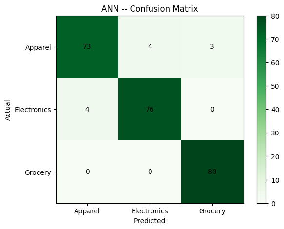
cm_ann = confusion_matrix(y_test, y_pred_ann)

fig, ax = plt.subplots()
im = ax.imshow(cm_ann, cmap="Greens")
ax.set_xticks(range(len(class_names))); ax.set_xticklabels(class_names)
ax.set_yticks(range(len(class_names))); ax.set_yticklabels(class_names)
ax.set_xlabel("Predicted"); ax.set_ylabel("Actual")
ax.set_title("ANN -- Confusion Matrix")
for i in range(len(class_names)):
    for j in range(len(class_names)):
        ax.text(j, i, cm_ann[i, j], ha="center", va="center")
plt.colorbar(im)
plt.show()

Task 4 : Why This Problem Needed a Neural Network

You've built a Perceptron and an ANN. Now use Logistic Regression, the traditional ML model used in the original scenario, to confirm that it also has a linear decision-boundary limitation.

Run Logistic Regression on the SmartCart Dataset

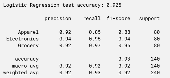
log_reg = LogisticRegression(max_iter=2000)
log_reg.fit(X_train_scaled, y_train)
y_pred_logreg = log_reg.predict(X_test_scaled)
logreg_acc = accuracy_score(y_test, y_pred_logreg)

print(f"Logistic Regression test accuracy: {logreg_acc:.3f}\n")
print(classification_report(y_test, y_pred_logreg, target_names=class_names))

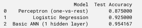
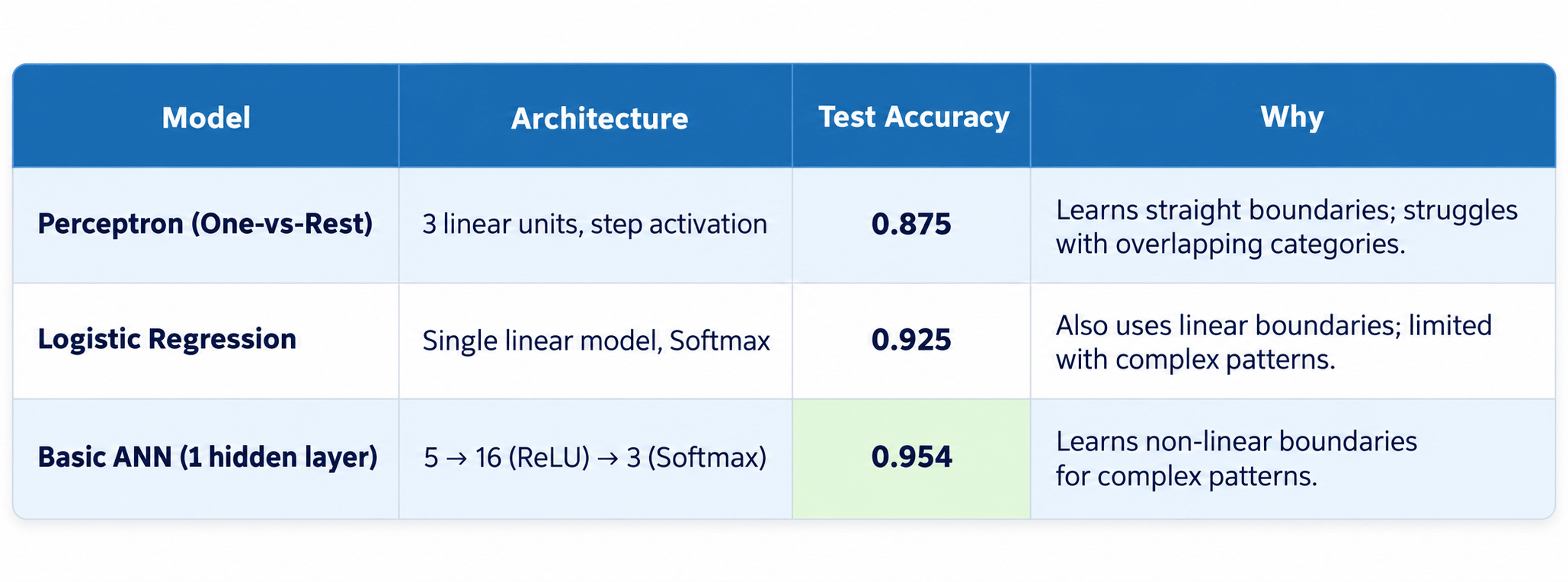
Compare all 3 Models

comparison = pd.DataFrame({
    "Model": ["Perceptron (one-vs-rest)", "Logistic Regression", 
    "Basic ANN (1 hidden layer)"],
    "Test Accuracy": [perceptron_acc, logreg_acc, ann_acc]})
comparison

Great job!

You have successfully compared Deep Learning with traditional Machine Learning, built and evaluated a Perceptron from scratch using SmartCart product data, learned the key building blocks of an ANN—layers, weights, bias, and activation functions—and built a basic ANN from scratch, comparing its performance with the Perceptron and Logistic Regression using actual results.

Checkpoint

Git Push

git push origin branchName

Next-Lab Preparation

Topic : Backpropagation and Gradient Descent

1) Loss Function
2) Gradients, Gradient Descent
3) Backpropagation Flow
4) Epochs & Convergence

GenAI - 1

GenAI - 1

Content ITV PRO

GenAI - 1

GenAI - 1

Content ITV PRO

More from Content ITV