Applied Measure Theory
for Probabilistic Modeling
Chad Scherrer
July 2023
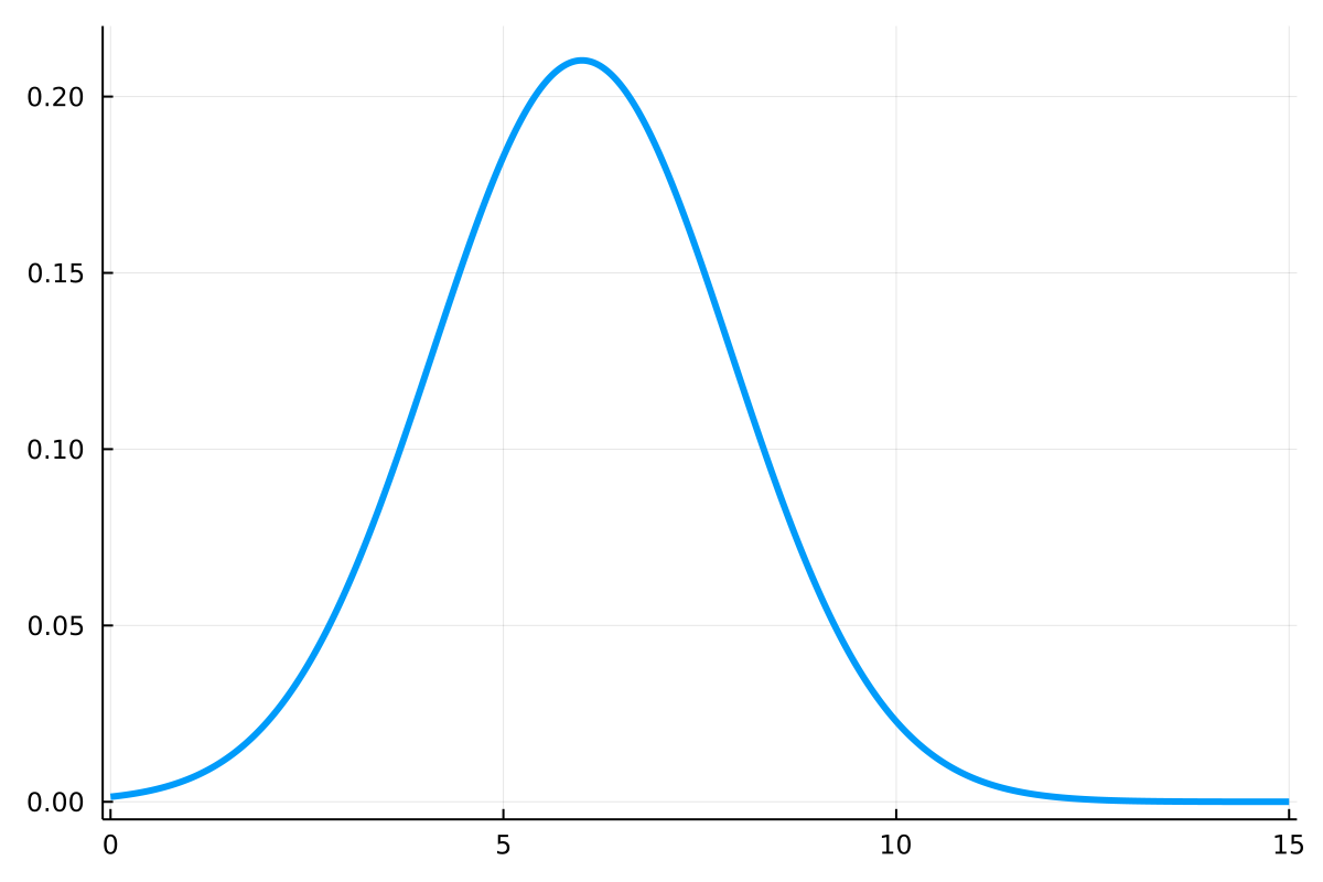
Motivation: Discrete vs Continuous Distributions
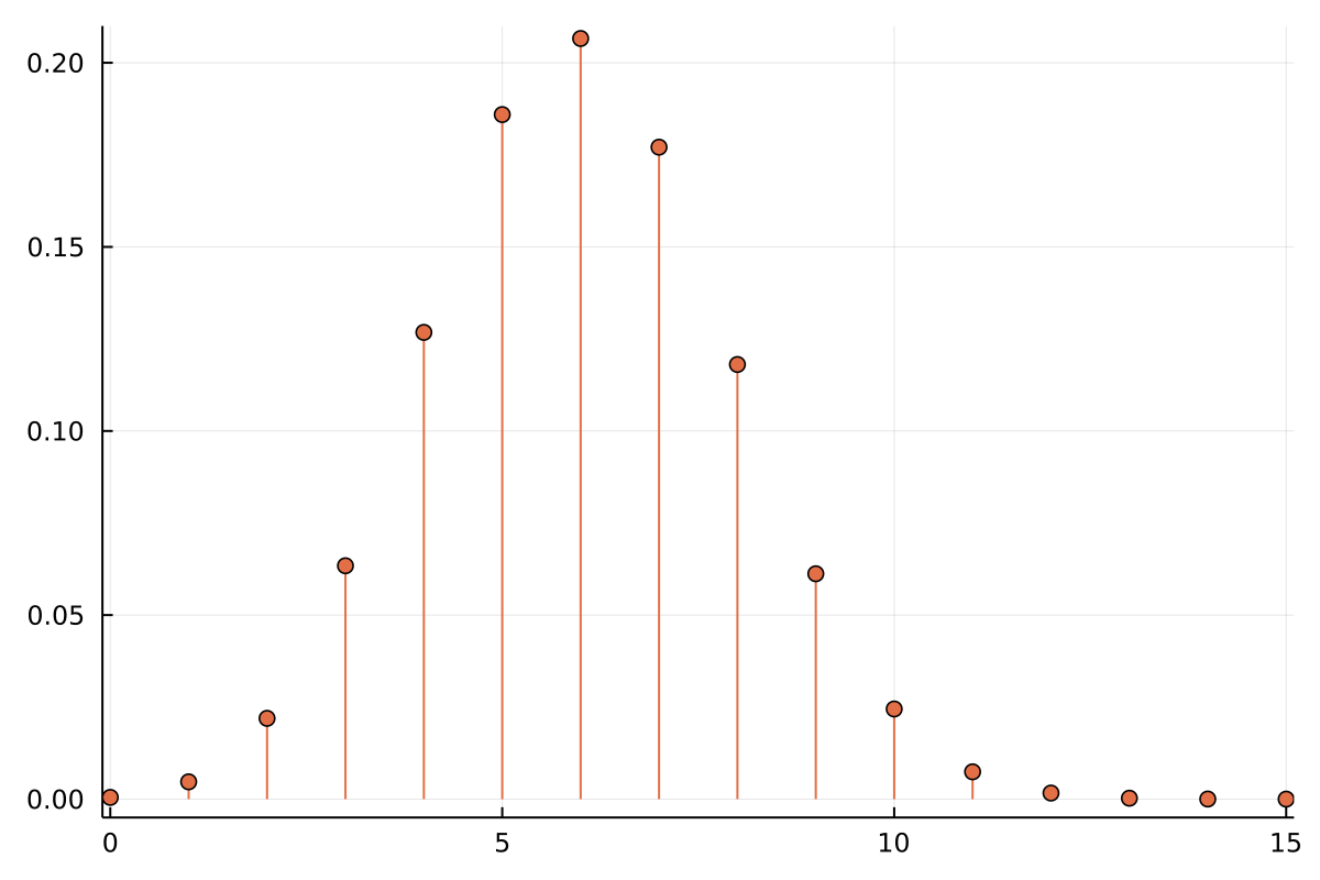
Discrete Distributions
- Expressed as a probability mass function
- Evaluation gives a probability
- Values sum to one
Continuous Distributions
- Expressed as a probability density function
- Evaluation gives a probability density
- Values integrate to one
\sum_j f(x_j) = 1
\int_{-\infty}^\infty f(x)\ dx = 1
Motivation: Discrete vs Continuous Distributions
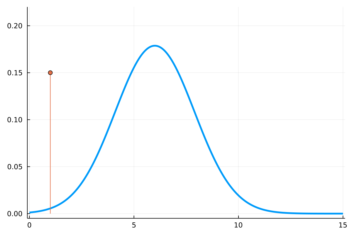
Discrete/Continuous Mixtures
- What is ?
- How is it interpreted?
- What is "integration"?
- How do we compute this?
f
discrete_part = Dirac(1)
continuous_part = Normal(15 * 0.4, sqrt(15 * 0.4 * 0.6))

m = 0.15 * discrete_part + 0.85 * continuous_part
In MeasureTheory.jl:
Importance Sampling
\text{To approximate } \mathbb{E}_{x \sim p}\left[ f(x) \right]
\text{Choose some proposal, } q(x)
\text{Then approximate } \mathbb{E}_{x \sim q}\left[ f(x) {\color{red} \frac{p(x)}{q(x)}} \right]
Rejection Sampling
\text{To sample from unnormalized } \tilde{p}(x)
\text{Accept when } M u < {\color{red} \frac{\tilde{p}(x)}{q(x)}} \text{, otherwise reject}
\text{Find sampleable } q(x) \text{, and } M \text{ such that } {\color{red} \frac{\tilde{p}(x)}{q(x)}} \le M
\text{Sample } u \sim \text{Uniform, and } x \sim q
Metropolis Hastings Sampling
\text{Sample } u \sim \text{Uniform, and } x' \sim q(x' \mid x)
\text{Accept when } u <
\left.
{\color{red}
\frac{\tilde{p}(x')}{q(x'\mid x)}
}
\middle/
{\color{red}
\frac{\tilde{p}(x)}{q(x\mid x')}
}
\right.
\text{, otherwise reject}
\text{Given sample } x \text{ and proposal } q(x' \mid x),
KL Divergence
\text{KL}(p\; \|\; q) = \mathbb{E}_{x\sim p}\left[ {\color{red} \frac{p(x)}{q(x)}} \right]
\text{Given ``true'' distribution } p
\text{ and approximating distribution } q,
What's really going on?
\frac{p(x)}{q(x)} \text{ is really } \frac{dp}{dq}(x) = \left. \frac{dp}{d\lambda}(x) \middle/ \frac{dq}{d\lambda}(x) \right.
p
q
\lambda
Densities are always relative!
The MeasureTheory.jl Approach
Densities are always relative
- Old and very standard idea (Lebesgue, Radon, Nikodym)
- But no other software we know of makes this explicit!
function basemeasure(::Normal{()})
  WeightedMeasure(static(-0.5 * log2π), LebesgueMeasure())
end

function logdensity_def(d::Normal{()}, x)
  -x^2 / 2
end
Computational advantages
- Easily represent more complex measures than usually possible
- Common structure can share computation
- Static computation makes this fast
- But no other software we know of makes this explicit!
Each measure has a base measure...
.. and a log-density relative to that base measure
Computing Log-Densities

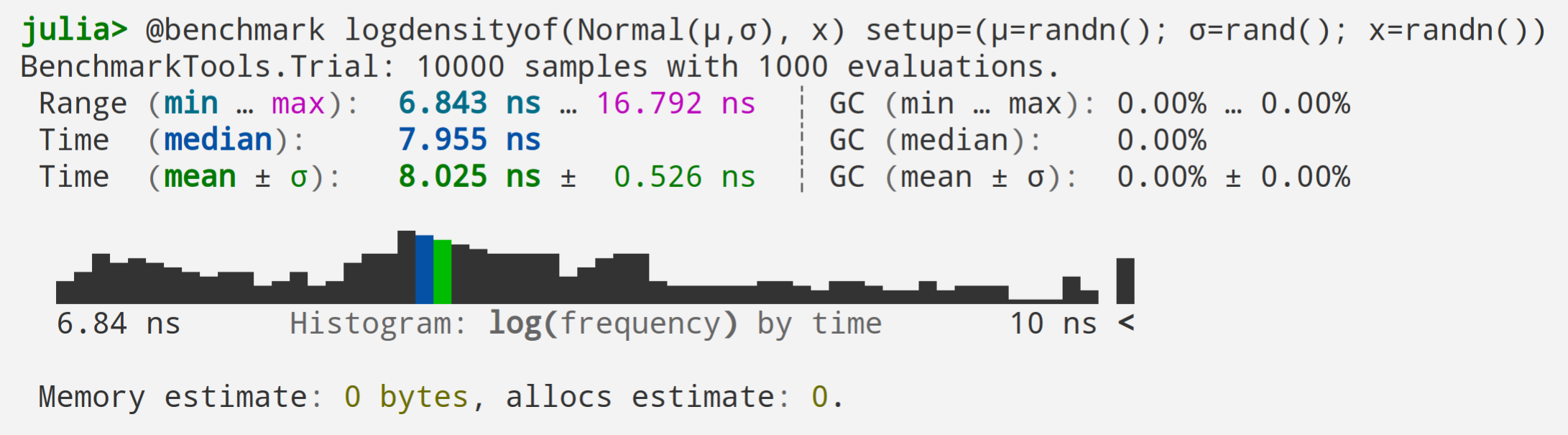
What actually happens when you call logdensityof(Normal(5,2), 1)?
Affine((μ=5, σ=2), Normal())
Normal(5,2)
proxy
insupport(Affine(...), 1)
✓
0.5 * LebesgueMeasure()
basemeasure
LebesgueMeasure()
basemeasure
ℓ == -3.6121
basemeasure
0.3989 * Affine((μ=5, σ=2), LebesgueMeasure())
\frac{1}{\sqrt{2 \pi}} \approx
ℓ = 0.0
ℓ += -2.0
-\frac{1}{2}\left(\frac{x-\mu}{\sigma}\right)^2
ℓ += -0.9189
\log \frac{1}{\sqrt{2 \pi}} \approx
ℓ += -0.6931
\log \frac{1}{2} \approx
Can This be Fast?
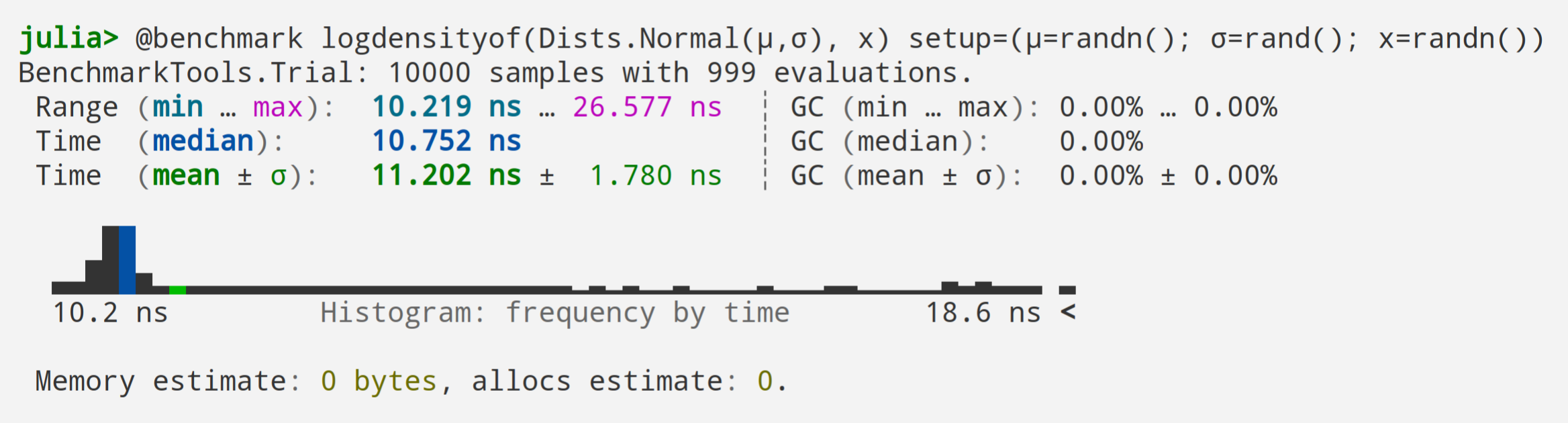
Distributions.jl
MeasureTheory.jl

Computing Relative Log-Density
\text{Lebesgue}(\mathbb{R})
\text{Beta}(\alpha, \beta)
\frac{1}{\sqrt{2\pi}}\text{Lebesgue}(\mathbb{R})
\text{Normal}(\mu, \sigma^2)
\text{Lebesgue}(\mathbb{I})
+
—
+
—
Parameterized Measures
Ways of writing Normal(0,2)
-\log {\color{darkorange} \sigma} - \frac{1}{2}\left(\frac{x - \color{blue} \mu}{\color{darkorange} \sigma}\right)^2
Normal(0,2)
Normal(μ=0, σ=2)
Normal(σ=2)
Normal(mean=0, std=2)
Normal(mu=0, sigma=2)
\frac{1}{2} \left( \log({\color{darkorange} τ}) - {\color{darkorange} τ} (x - {\color{blue} μ})^2 \right)
Normal(μ=0, τ=0.25)-\frac{1}{2} \left( \log {\color{darkorange} \sigma^2} - \frac{(x - {\color{blue} \mu})^2}{\color{darkorange} \sigma^2} \right)
Normal(μ=0, σ²=4)
Normal(mean=0, var=4)
-{\color{darkorange} \log \sigma} - \frac{(x - {\color{blue} μ})^2}{2 e^{2 {\color{darkorange} \log \sigma}}}
Normal(μ=0, logσ=0.69)Defining New Measures
A measure can be primitive or defined in terms of existing measures
Primitive Measures
TrivialMeasureLebesgueMeasureCountingMeasure
Product-like
-
ProductMeasure(⊗) -
PowerMeasure(^) For
Sum-like
-
SuperpositionMeasure(+) SpikeMixture-
IfElseMeasure(IfElse.ifelse)
Transformed Measures
-
PushforwardMeasure(pushfwd) -
Affine(affine)
Density-related
-
WeightedMeasure(*) -
PowerWeightedMeasure(↑) -
PointwiseProductMeasure(⊙) ParameterizedMeasure-
DensityMeasure(∫)
Support-related
-
RestrictedMeasure(restrict) -
HalfMeasure(Half) Dirac
IID Products

d = Beta(2,4) ^ (40,64)A PowerMeasure produces replicates a given measure over some shape.
⋆
⋆Independent and Identically Distributed
Products with Index Dependence

d = For(40,64) do i,j
    Beta(i,j)
end
For(indices) do j
# maybe more computations
# ...
some_measure(j)
endFor produces independent samples with varying parameters.
Markov Chains

mc = Chain(Normal(μ=0.0)) do x Normal(μ=x) end
r = rand(mc)
Define a new chain, take a sample
julia> take(r,100) == take(r,100)
true
This returns a deterministic iterator
julia> logdensityof(mc, take(r, 1000))
-517.0515965372
Evaluate on any finite subsequence
Working with Likelihoods
prior = HalfNormal()

\begin{aligned}
\color{#009cfa} \sigma &\color{#009cfa}\sim \text{Normal}_+(0,1) \\
\phantom{\color{#e47045} x_n} &\phantom{\color{#e47045} \sim \text{Normal}(0,\sigma}
\end{aligned}
Working with Likelihoods
prior = HalfNormal()

d = Normal(σ=2.0) ^ 10
lik = likelihood(d, x)

\begin{aligned}
\color{#009cfa} \sigma &\color{#009cfa}\sim \text{Normal}_+(0,1) \\
\color{#e47045} x_n &\color{#e47045} \sim \text{Normal}(0,\sigma)
\end{aligned}
Working with Likelihoods
prior = HalfNormal()

d = Normal(σ=2.0) ^ 10
lik = likelihood(d, x)

post = prior ⊙ lik
\begin{aligned}
\color{#009cfa} \sigma &\color{#009cfa}\sim \text{Normal}_+(0,1) \\
\color{#e47045} x_n &\color{#e47045} \sim \text{Normal}(0,\sigma)
\end{aligned}
{\color{#3ba64c} P(\sigma | x)} \propto {\color{#009cfa} P(\sigma)} {\color{#e47045} P(x | \sigma)}
Symbolic Evaluations
julia> using MeasureTheory, Symbolics

julia> @variables μ τ
2-element Vector{Num}:
 μ
 τ

julia> d = Normal(μ=μ, τ=τ) ^ 1000;

julia> x = randn(1000);

julia> ℓ = logdensityof(d, x) |> expand
500.0log(τ) + 3.81μ*τ - (503.81τ) - (500.0τ*(μ^2))- Types and functions are generic, so symbolic manipulations work out of the box
- Compare
- MeasureTheory.jl
- Distributions.jl
julia> logdensityof(Distributions.Normal(μ, 1 / √τ), 2.0)
ERROR: MethodError: no method matching logdensityof(::Num, ::Float64)
Packages Using MeasureTheory.jl
- bat/BAT.jl: A Bayesian Analysis Toolkit in Julia (v3 will use MeasureBase.jl)
-
cscherrer/DistributionMeasures.jl: Conversions between Distributions.jl distributions and MeasureTheory.jl measures.
-
cscherrer/Soss.jl: Probabilistic programming via source rewriting
-
cscherrer/Tilde.jl: WIP successor to Soss.jl
-
jeremiahpslewis/IteratedProcessSimulations.jl: Simulate Machine Learning-based Business Processes in Julia
-
JuliaGaussianProcesses/AugmentedGPLikelihoods.jl: Provide all functions needed to work with augmented likelihoods (conditionally conjugate with Gaussians)
- mschauer/Mitosis.jl: Automatic probabilistic programming for scientific machine learning and dynamical models
-
mschauer/MitosisStochasticDiffEq.jl: Backward-filtering forward-guiding with StochasticDiffEq.jl
-
oschulz/ValueShapes.jl: Duality of view between named variables and flat vectors in Julia
-
ptiede/Comrade.jl: Composable Modeling of Radio Emission
-
ptiede/HyperCubeTransform.jl: We love to use nested sampling with the EHT, but it is rather annoying to
constantly write the prior transformation. This package will do that for you.
Thank You!
2023-06-MeasureTheory-Munich
By Chad Scherrer


