Deep equals Shallow in Kernel Regimes
Study Group on Learning Theory
Daniel Yukimura

and some more...
Previously...
- Deep Neural Networks (DNN) are universal approximators
-
Challenges:
- Non-convex optimization.
- Generalization + Overparameterization.
-
Neural Tangent Kernels (NTK):
- Under certain conditions overparameterized DNNs are equivalent to kernel methods.
- Successful optimization!
So... is deep learning solved?
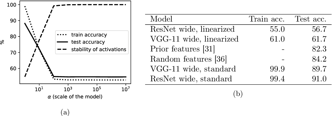
- Perfomance gap between NNs and NTKs:
- 5-7% in favor of DNNs on CIFAR-10
- NTKs outperform DNNs on small datasets
- Larger gap for ResNet
- Depends on the task complexity
- DNNs approximate better some classes of functions
- Depth doesn't matter much for NTKs
Deep equals shallow for ReLU Networks in Kernel Regimes
Result: Kernels derived from DNNs have the same approximation properties than shallow networks.
Consequence: The Kernel framework doesn't seem to explain the benefits of deep architectures.
Approx. using dot-product kernels:
\bullet \hspace{2mm} \text{Consider the shallow case: } f(x) = \frac{1}{\sqrt{m}} \sum\limits_{j=1}^m v_j \sigma( w_j^\intercal x)
Random feature kernels:
k(x,x') = \mathbb{E}_{w\sim \mathcal{N}(0,I)} [\sigma(w^\intercal x) \sigma(w^\intercal x')]
\bullet \hspace{2mm} \text{When only the } (v_j)_j \text{ are trained (with }\ell_2 \text{ reg.)}
\Rightarrow \text{ random feature approx.}
\bullet \hspace{2mm} \text{If } x, x' \text{ are on the sphere, then}
k(x,x') = \kappa(x^\intercal x')
\bullet \hspace{2mm} \text{If we decompose }\sigma\text{ using hermite poly.}
\Rightarrow \kappa(u) = \sum\limits_{i\geq 0} a_i^2 u^i
\text{for some }\kappa.
\sigma(u) = \displaystyle\sum\limits_{i\geq 0} a_i h_i(u)
orth. for the Gaussian meas.
\bullet \hspace{2mm} \text{Usefull }\kappa\text{s:}
\kappa_0(u) = \dfrac{1}{\pi}(\pi - \arccos(u))
\kappa_1(u) = \dfrac{1}{\pi}\left( u (\pi - \arccos(u)) + \sqrt{1-u^2} \right)
Step func.
ReLU
Neural Tangent Kernels:
f(x,\theta) \approx f(x,\theta_0) + \left<\theta - \theta_0, \nabla_\theta f(x,\theta_0)\right>
f(x,\theta) = \sigma( W_L \sigma(\dots W_2\sigma(W_1 x)))
\bullet \hspace{2mm} \text{Deep networks}
\bullet \hspace{2mm} \text{Overparam. regime and } W^\ell_{i,j} \sim \mathcal{N}\left(0, \frac{1}{n_\ell}\right)
k_{NTK} (x,x') = \lim\limits_{m\rightarrow \infty} \left< \nabla f(x, \theta_0), \nabla f(x', \theta_0) \right>
\Rightarrow
\bullet \hspace{2mm} \text{If our inputs are on the sphere:}
k_{NTK} (x,x') = \kappa^L_{NTK}(x^\intercal x')
\kappa^1_{NTK}(x,x') = \kappa^1(u) = u
\kappa^\ell(u) = \kappa_1( \kappa^{\ell-1}(u) )
\kappa^\ell_{NTK}(u) = \kappa^{\ell-1}_{NTK}(u) \kappa_0\left(\kappa^{\ell-1}(u)\right) + \kappa^\ell(u)
\text{defined recursively as:}
\text{for }\ell = 2,\dots,L
Spherical harmonics and description of the RKHS
\bullet \hspace{2mm} \text{Consider the integral operator } T
T f(x) = \displaystyle\int k(x,y) f(y) d \tau (y)
\bullet \hspace{2mm} \text{ In the sphere we can diag. }\kappa \text{ using spher. harmonics}
T Y_{k,j} = \mu_k Y_{k,j}
\text{j-th spher. harmonic poly. of degree k}
\text{eigenvalues}
\text{uniform on }\mathbb{S}^{d-1}
N(d,k) = \frac{2k+d-2}{k} \binom{k+d-3}{d-2}
\sim \mathcal{O} \left( k^{d-2} \right)
\bullet \hspace{2mm} \# \text{ spheric harmonics of degree }k:
\bullet \hspace{2mm} \text{ RKHS space associated to the kernel:}
\text{surface area of }\mathbb{S}^{d-1}
\bullet \hspace{2mm} \text{Eigenvalues:}
\mu_k = \dfrac{\omega_{d-2}}{\omega_{d-1}} \displaystyle\int\limits_{-1}^1 \kappa(t) P_k(t) (1-t^2)^{\frac{(d-3)}{2}} dt
\mathcal{H} = \left\{ f =\displaystyle\sum\limits_{k\geq 0, \mu_k\neq 0} \sum\limits_{j=1}^{N(d,k)} a_{k,j} Y_{k,j}(\cdot), \text{ s.t. }
\|f\|_{\mathcal{H}}^2 = \sum\limits_{k\geq 0, \mu_k\neq 0} \sum\limits_{j=1}^{N(d,k)} \frac{a_{k,j}^2}{\mu_{k}} < \infty \right\}
\text{if }\mu_k\text{ has a fast decay}
\Rightarrow a_{k,j} \text{ must also decay quickly}
\text{Legendre poly. of degree }k
\textbf{Theorem 1:}\text{(Decay from regularity of }\kappa\text{ at endpoints)}
\text{Let } \kappa:[-1,1] \rightarrow \mathbb{R} \text{ be a function } C^\infty\text{ at }(-1,1)
\text{and around } \pm 1 \text{ we have}:
\kappa(1-t) = p_1(t) + c_1 t^\nu + \mathcal{o}(t^\nu)
\kappa(-1+t) = p_{-1}(t) + c_{-1} t^\nu + \mathcal{o}(t^\nu)
\text{for } t\geq 0,\hspace{2mm} p_1, p_{-1} \text{ poly., and } \nu\notin \mathbb{Z}.
\text{Then, there's an absolute const. }C(d,\nu)\text{ s.t.:}
\bullet \hspace{2mm} \text{ For k even, if }c_1\neq c_{-1}: \hspace{3mm} \mu_k \sim (c_1+c_{-1}) C(d,\nu) k^{-d - 2\nu +1}
\bullet \hspace{2mm} \text{ For k odd, if }c_1\neq c_{-1}: \hspace{3mm} \mu_k \sim (c_1 - c_{-1}) C(d,\nu) k^{-d - 2\nu +1}
Consequences for ReLU networks:
\kappa_0 (1-t) = 1 - \frac{\sqrt{2}}{\pi} t^{1/2} + \mathcal{O}(t^{3/2})
\kappa_1 (1-t) = 1 - t + \frac{2\sqrt{2}}{3 \pi} t^{3/2} + \mathcal{O}(t^{5/2})
\bullet \hspace{2mm} \text{similarly around} -1\dots
\bullet \hspace{2mm} \text{Expansions around} +1
\text{From theorem 1} \Rightarrow
\bullet \hspace{2mm} \text{A decay of } k^{-d-2}\text{ for even coeff. of }\kappa_1
\bullet \hspace{2mm} \text{A decay of } k^{-d}\text{ for odd coeff. of }\kappa_0
\textbf{Corollary 3:}\text{(Deep NTK decay)}
\text{For the } \kappa_{NTK}^L \text{of an L-layer ReLU network with } L\geq 3
\text{we have } \mu_k \sim C(d,L) k^{-d}, \text{ where }C(d,L) \text{ differs with the}
\text{parity of }k \text{ and grows quadratically with } L.
\bullet \hspace{2mm} \text{A similar result holds for random feature approx.}
\bullet \hspace{2mm} \text{Shows that NTKs has the same decay as Laplace kernels}
\bullet \hspace{2mm} \text{DNNs with the step activation improve with depth.}
\bullet \hspace{2mm} \text{Kernels assoc. with }C^\infty \text{activations have decay faster}
\text{than any poly.}\Rightarrow \text{RKHS contains only smooth functions}
What else?
- Lazy vs Active regimes:
\Rightarrow
\text{lazy training} \sim \text{linearization}
\Delta(L) >> \Delta(Df)
\text{ loss }
\text{ model grad. }

\Rightarrow
some DNNs might have lazy behavior, but the good ones are not on this regime.
What else?
- Taylorized Training:

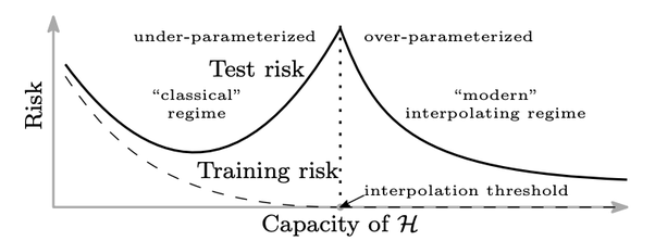
- Double descent curve:

\text{ initial evidence }
\text{ using NTKs }
\text{ random features }
- Hierarchical Learning:
\text{ Backward Feature Correction }
A learner learns a complicated target by decomposing it into a sequence of simpler functions.
\text{ Neural representations }
- Hierarchical learning seems to be an important property of DNNs.
- Hierarchical learning is not leveraged by NTKs
Deep equals Shallow for NTKs
By Daniel Yukimura
Deep equals Shallow for NTKs
- 458


