Differentiable Rendering

Daniel Yukimura

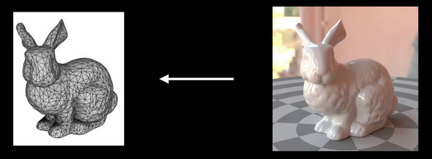
scene

parameters

2D image

  • camera pose
  • geometry
  • materials
  • lighting
  • ...

rendering

scene

parameters

2D image

rendering

rendering

differentiable

Feedback

Learning

  • Inverse Graphics
  • Optimization
  • 3D Reconstruction
  • Fast rendering
  • ...

Applications:

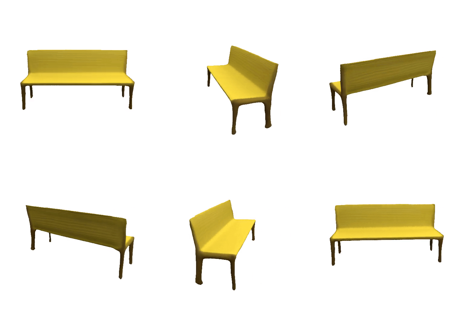
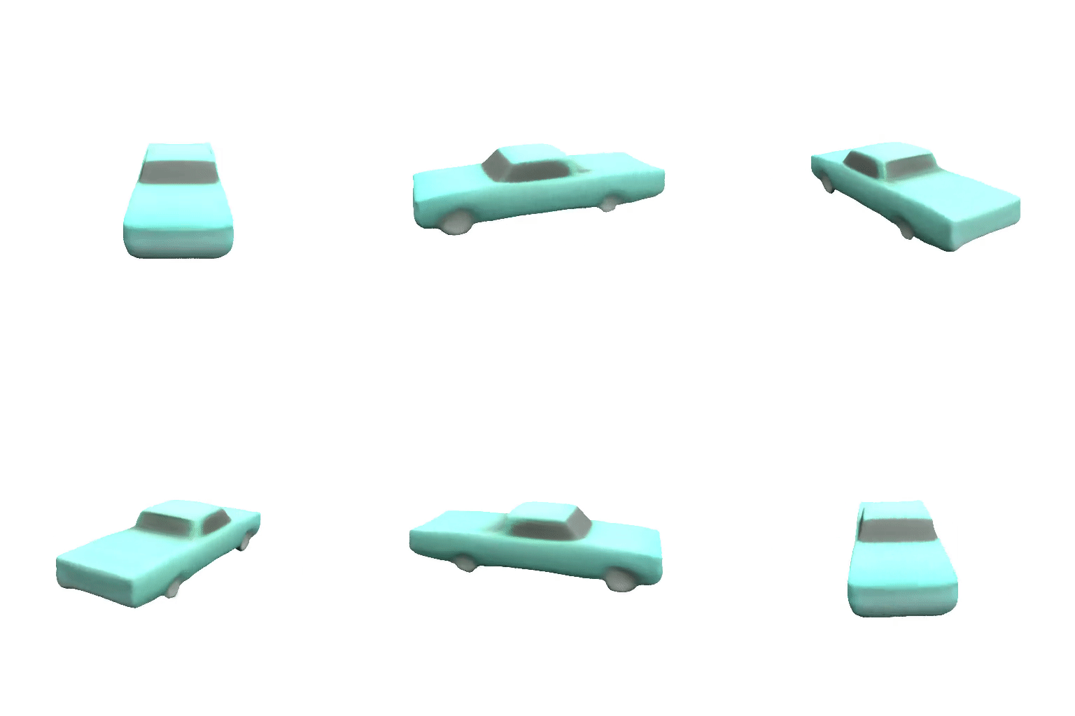
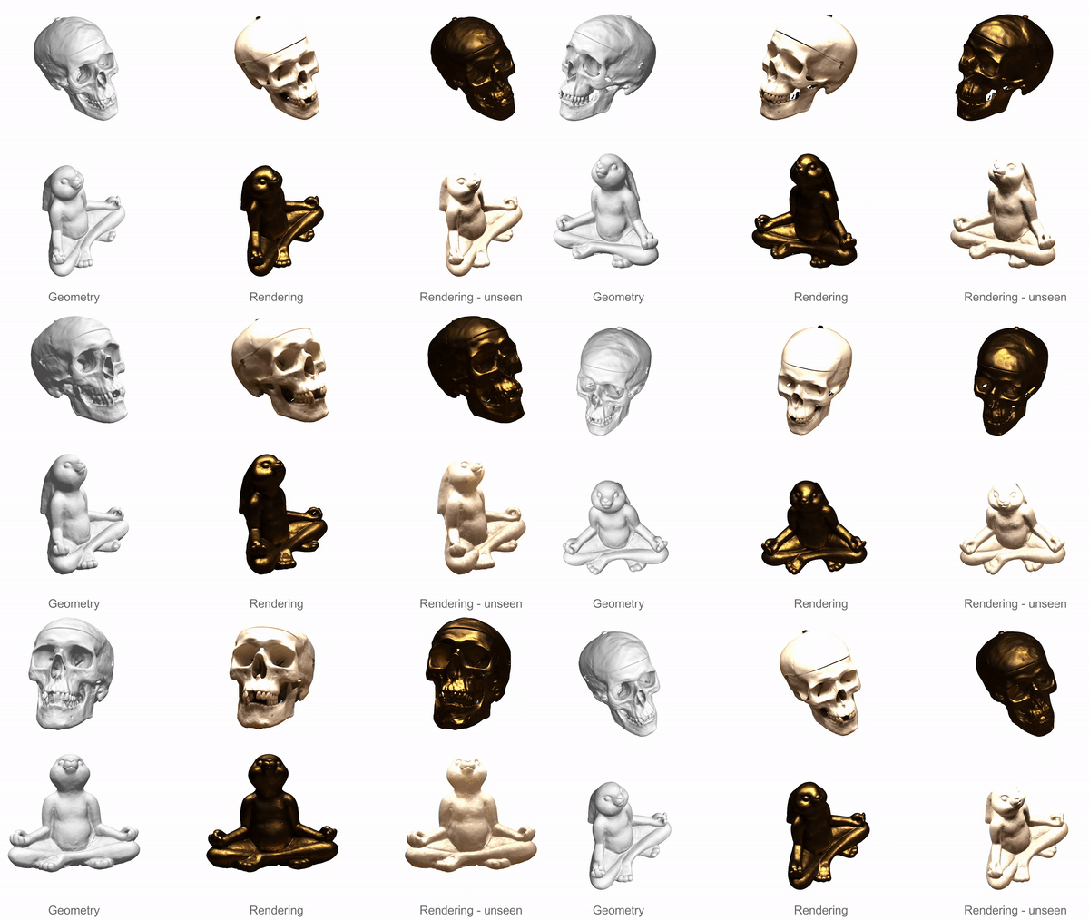
Wang Yifan, Felice Serena, Shihao Wu, Cengiz Öztireli, Olga Sorkine-Hornung - ACM SIGGRAPH ASIA 2019.
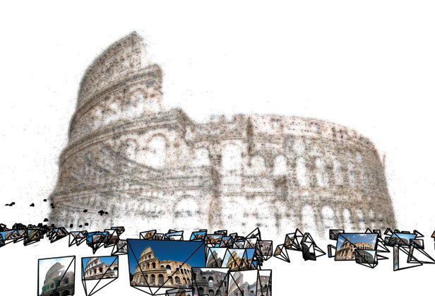
Sameer Agarwal, Noah Snavely, Ian Simon, Steven M. Seitz and Richard Szeliski - International Conference on Computer Vision, 2009, Kyoto, Japan.
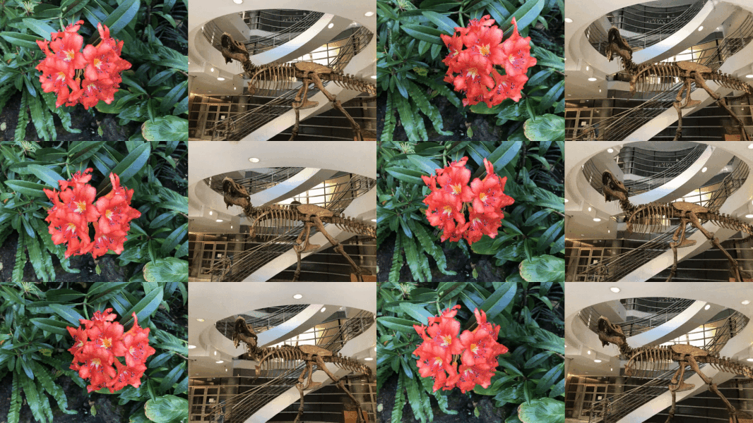
Differentiable Monte Carlo Ray Tracing through Edge Sampling

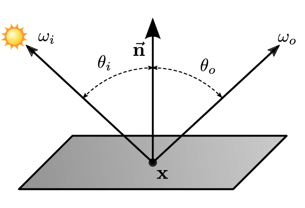
L_o(x, \vec \omega) = L_e(x, \vec \omega) + \displaystyle\int_{\Omega} L_i(x,\vec \omega')f_r(\vec \omega, x, \vec \omega') \cos(\theta) d\vec\omega'

Rendering equation:

Global Illumination

(Recalling)
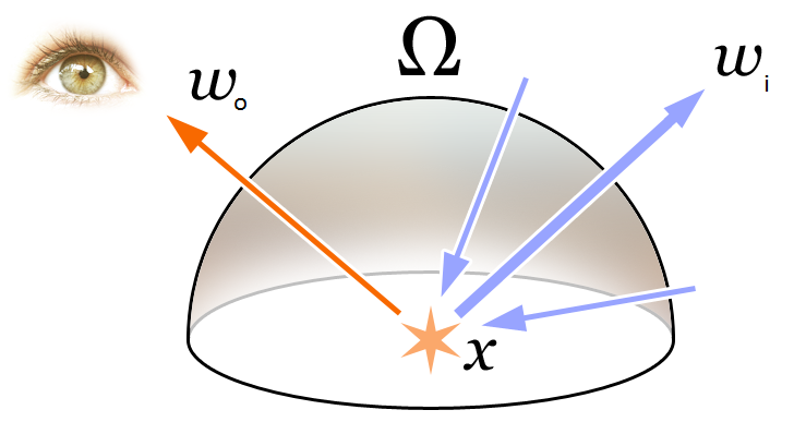
Monte Carlo Integration

(Recalling)
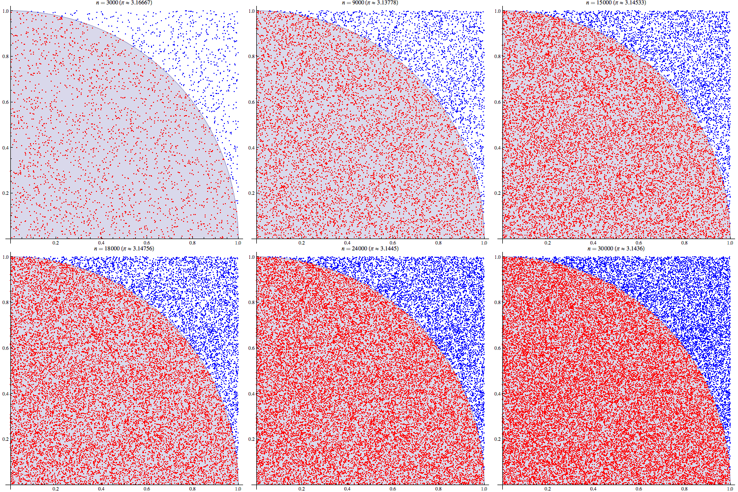
\displaystyle\int f(x) dx = ?
\mathbb{E}\left[f(X)\right] = \displaystyle\int f(x) p(x) dx
\approx \frac{1}{N} \sum\limits_{i=1}^N f(X_i)
\text{(LLN)}
X_i \sim p(\cdot)
\displaystyle\int f(x) dx = \displaystyle\int f(x)\frac{p(x)}{p(x)} dx
= \mathbb{E}\left[ \frac{f(X)}{p(X)} \right]
\approx \frac{1}{N} \sum\limits_{i=1}^N \frac{f(X_i)}{p(X_i)}

Monte Carlo Integration

(Recalling)

\displaystyle\int_{\Omega} L_i(x,\vec \omega')f_r(\vec \omega, x, \vec \omega') \cos(\theta) d\vec\omega' \approx \frac{1}{N}\sum\limits_{i=1}^N \dfrac{L_i(x,\vec \omega_i')f_r(\vec \omega, x, \vec \omega_i') \cos(\theta) d\vec\omega_i'}{p(\vec\omega_i')}

Path Tracing

(Recalling)

Differentiable Monte Carlo Ray Tracing through Edge Sampling

\text{Parameter set } \Phi
  • camera pose
  • geometry
  • materials
  • lighting
  • ...
\text{Path Tracing}
I
f(I)
\text{(image)}
\text{scalar function}\\ \text{e.g. loss function}
\text{Goal: Differentiate/Backpropagate}

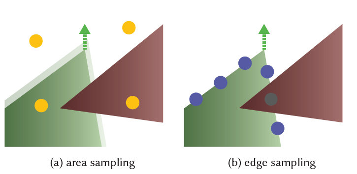
Strategy: Break into smooth and discontinuous regions.

L_i(p) = \displaystyle\int_{\mathcal{M}} {\ell_i( p \leftarrow m ) d A(m)}
= (S_i) + (D_i)
S_i \rightarrow \text{tradicional area sampling }
+ \text{ auto-differentiation}
D_i \rightarrow \text{Edge Sampling}

Assumptions:

  • triangular meshes (with no interpenetration)
  • no point light sources
  • no perfectly specular surfaces

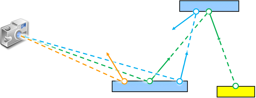
Primary visibility

(2D screen-space domain)
I = \displaystyle\int \hspace{-1mm}\displaystyle\int k(x,y) L(x,y) dx dy
\text{pixel color}
\text{pixel filter}
\text{radiance}
f(x,y) = k(x,y) L(x,y)
\textbf{Goal: } \nabla I = \nabla \displaystyle\int \hspace{-1mm}\displaystyle\int f(x,y;\Phi) dx dy
  • All discontinuities happen at triangle edges.
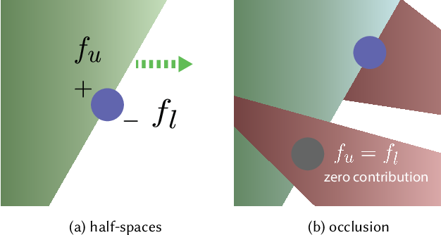
\bullet \hspace{2mm} \text{From an edge split the space in two: } f_u \text{ and } f_\ell
\alpha(x,y) > 0 \Rightarrow (x,y)\in f_u
\text{edge equation}
f(x,y) = \theta( \alpha(x,y) ) f_u(x, y) + \theta( -\alpha(x,y) ) f_\ell(x,y)
\text{step function}
\text{edge: } (a_x, a_y), (b_x, b_y)
\alpha(x,y) = (a_y - b_y)x + (b_x - a_x)y + (a_x b_y - b_x a_y)
f(x,y) = \displaystyle\sum\limits_{i} \theta( \alpha_i(x,y) ) f_i(x, y)
\nabla \displaystyle\int \hspace{-2mm}\displaystyle\int \theta( \alpha_i(x,y) ) f_i(x, y) d_x d_y = \displaystyle\int \hspace{-2mm}\displaystyle\int \theta(\alpha_i(x,y)) \nabla f_i(x,y) dx dy
+ \displaystyle\int \hspace{-2mm}\displaystyle\int \delta(\alpha_i(x,y)) \nabla \alpha_i(x,y) f_i(x,y) dx dy
\textbf{discontinuous}
\textbf{smooth}
\displaystyle\int \hspace{-2mm}\displaystyle\int \delta(\alpha_i(x,y)) \nabla \alpha_i(x,y) f_i(x,y) dx dy =
= \displaystyle\int \hspace{-4mm}\displaystyle\int\limits_{\alpha_i(x,y)=0} \dfrac{\nabla \alpha_i(x,y)}{\|\nabla_{x,y} \alpha_i(x,y)\|} \nabla \alpha_i(x,y) f_i(x,y) d\sigma (x,y)
\text{length measure}\\ \text{on the edge}
\displaystyle\int \hspace{-4mm}\displaystyle\int\limits_{\alpha_i(x,y)=0} \dfrac{\nabla \alpha_i(x,y)}{\|\nabla_{x,y} \alpha_i(x,y)\|} \nabla \alpha_i(x,y) f_i(x,y) d\sigma (x,y)

Monte Carlo estimation:

\approx \dfrac{1}{N} \displaystyle\sum\limits_{j=1}^N \dfrac{\|E\| \nabla \alpha_i(x_j,y_j) (f_u(x_j,y_j) - f_\ell(x_j, y_j)) }{ P(E) \|\nabla_{x,y} \alpha_i(x,y)\|}
\text{length of E}
\text{prob. of selec. E}

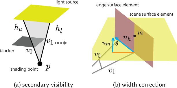
Secondary visibility

g(p) = \displaystyle \int_\mathcal{M} h(p, m) dA(m)

(global illumination - 3D)

\text{scene manifold}
\text{area measure}
\text{3D edge: } (v_0, v_1)
\theta( \alpha(p,m) ) h_u(p,m) + \theta( -\alpha(p,m) ) h_\ell(p,m)
\alpha(p, m) = (m - p)\cdot (v_0 - p) \times (v_1 - p)

edge portion:

\displaystyle \int\limits_{\alpha(p,m) = 0} \dfrac{\nabla \alpha(p,m)}{\|\nabla_m \alpha(p,m)\|} h(p,m) \dfrac{1}{\|n_m \times n_h\|} d\sigma' (m)
n_h = \dfrac{(v_0 - p)\times (v_1 - p)}{\|(v_0 - p)\times (v_1 - p)\|}

Importance Sampling The Edges

  • There are many triangles to sample.
  • Now we have to sample edges
  • and sample points from the edges...
  • Most edges are not silhouette
  • not all points have non-zero contribution

Hierarchical edge sampling

two hierarchies:

  1. Triangle edges that associate with only one face and meshes w/ no smooth shading.
  2. All the remaining edges

volume hierarchie:

  1. 3D bounding volume: 3D pos. of edge endpoints.
  2. 6D bounding volume: pos. of edge endpoints and the normals associated w/ the faces of the edge

Importance sampling a single edge

  • Sample based on the BRDF
  • Precompute a table of fitted linearly transformed cosines for all BRDFs.
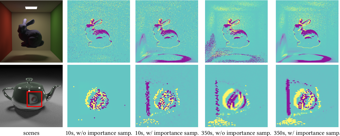
Results

Inverse rendering:

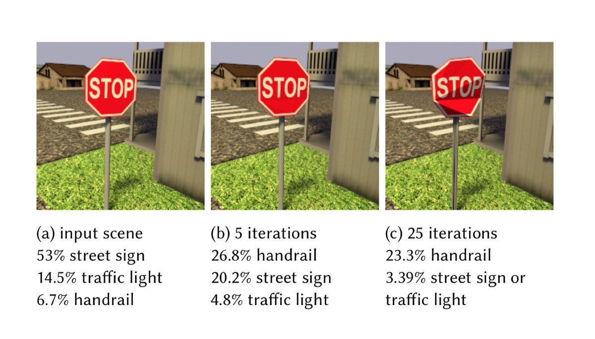
Adversarial examples:
Implicit Representation
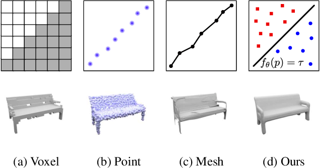
  • Do not represent 3D shape explicitly
  • Instead, consider it implicitly as decision boundary of a classifier

Occupancy networks

  • Represent the implicit surface as a neural network.
f_\theta: \mathbb{R}^3 \times \mathcal{Z} \rightarrow [0,1]
\text{3D location}
\text{Condition}
\text{occupancy}\\ \text{probability}

Differentiable Volumetric Rendering
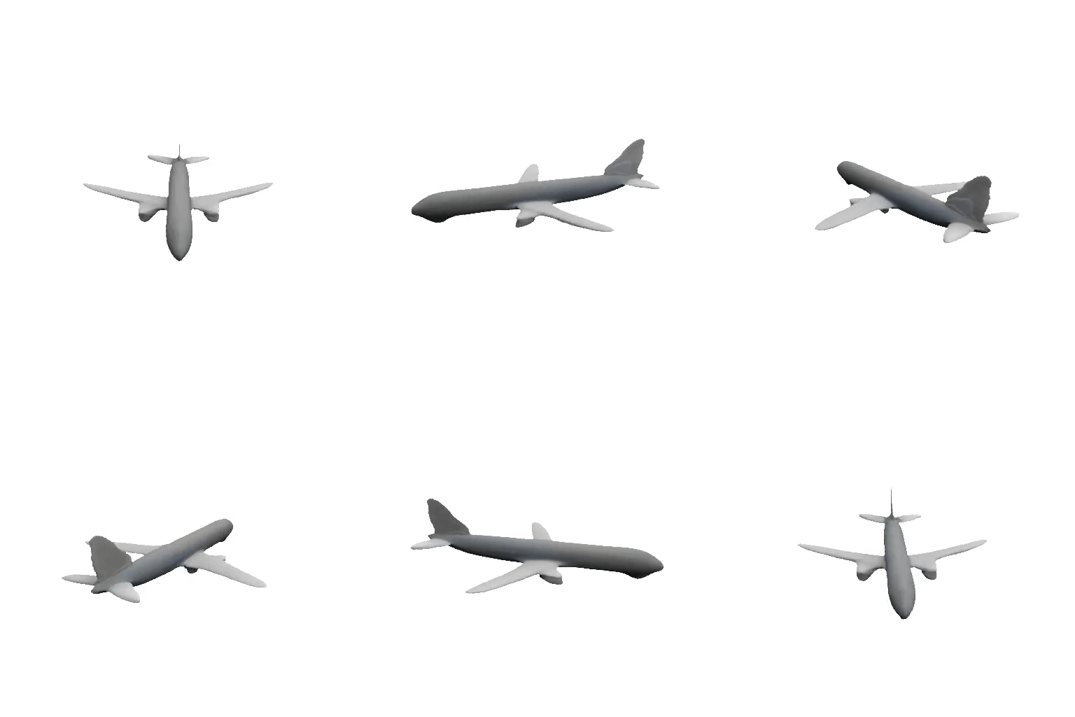
Architecture

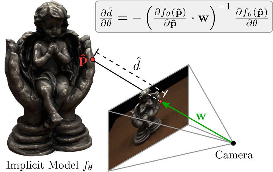
  • Volumetric Rendering is differentiable here!
  • Depth gradients

Forward Pass - Rendering:
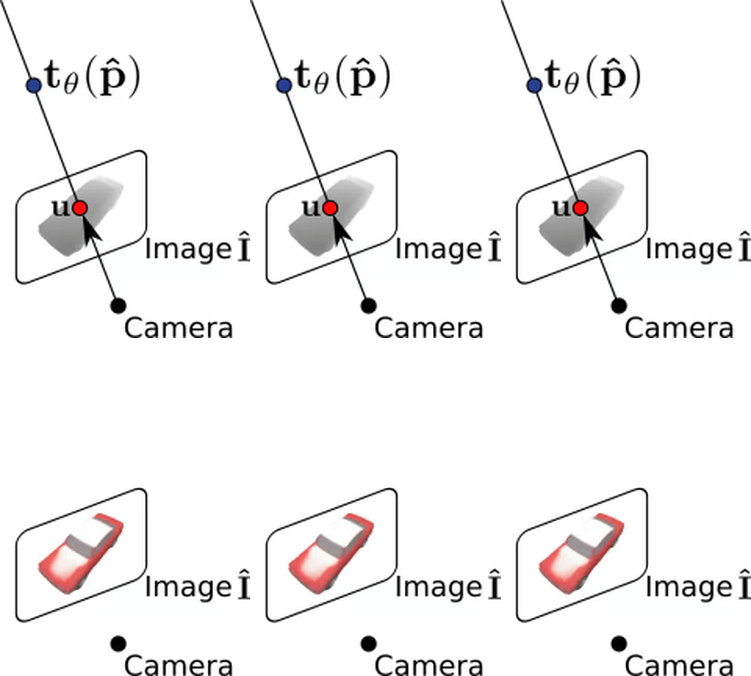
Texture mapping:
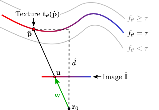
t_\theta: \mathbb{R}^3 \times \mathcal{Z} \rightarrow \mathbb{R}^3
\hat{p} = \text{``first interesection with } \{p\in \mathbb{R}^3 | f_\theta(p) = \tau \} \text{"}
\mathcal{L}(\hat{I}, I) = \sum\limits_u \|\hat{I}_u - I_u \|

Loss:

Differentiable Rendering:

\frac{\partial \mathcal{L}}{\partial\theta} = \sum\limits_u \frac{\partial \mathcal{L}}{\partial \hat{I}_u} \frac{\partial \hat{I}_u}{\partial \theta} \\
= \sum\limits_u \frac{\partial \mathcal{L}}{\partial \hat{I}_u} \frac{\partial t_\theta (\hat{p})}{\partial \theta} \frac{\partial \hat{p}}{\partial\theta}

KNOWN

??

Depth Gradients:

r(d) = r_0 + d w
\exists\hspace{2mm} \hat{d} \text{ s.t. } \hat{p} = r(\hat{d})
\text{depth}

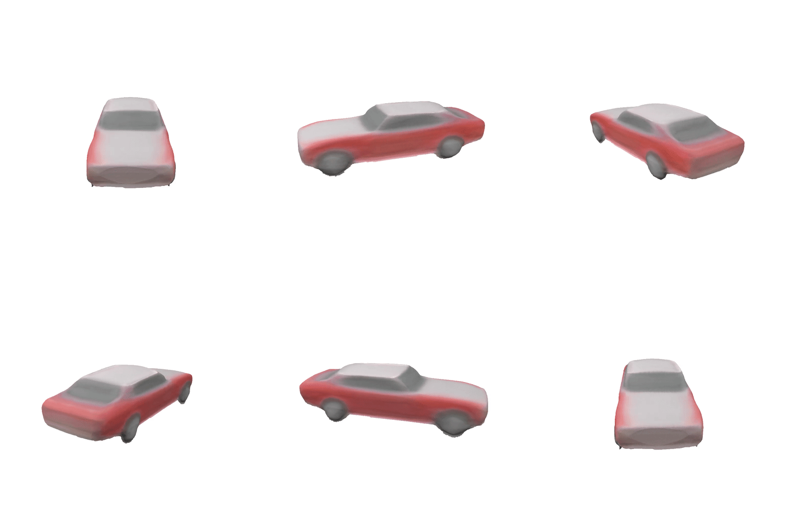
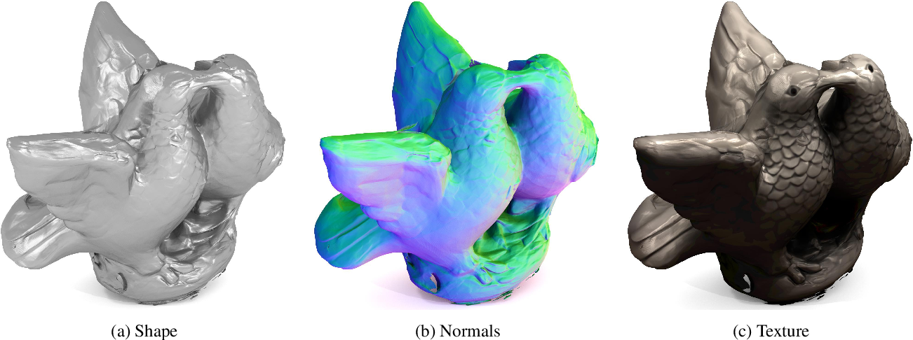
Results

Implicit Differentiable Rendering

Multiview 3D Surface Reconstruction

Input: Collection of 2D images (masked)

             with rough or noisy camera info.

Targets:

  • Geometry
  • Appearance (BRDF, lighting conditions)
  • Cameras

Method:

Geometry:

\mathcal{S}_\theta = \{ x\in \mathbb{R}^3 | f(x;\theta) = 0 \}

signed distance function (SDF) +

implicit geometric regularization (IGR)

\theta

- geometry parameters

IDR - Forward pass
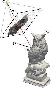
R_p(\tau) = \{ c_p + t v_p | t \geq 0 \}
\hat{x}_p = \hat{x}_p(\theta, \tau) = R_p(\tau) \cap \mathcal{S}_\theta
\tau \text{ - camera parameters}

Ray cast:

(first intersection)

p \text{ - pixel}

IDR - Forward pass

L_p(\theta, \gamma, \tau) = M(\hat{x}_p, \hat{n}_p, \hat{z}_p, v_p; \gamma)
\gamma

- appearance parameters

Output (Light Field):

Surface normal

\hat{n}_p(\theta)

Global gometry feature vector

\hat{z}_p(\hat{x}_p; \theta)

Differentiable intersections

\theta_0, \tau_0 - \text{current parameters}
\hat{x}(\theta, \tau) = c + t_0 v - \frac{v}{\nabla_x f(x_0; \theta_0) \cdot v_0} f(c + t_0 v; \theta)

Lemma:

Light Field Approx.

L(\hat{x}, w^o) = L^e(\hat{x}, w^o) + \int\limits_\Omega B(\hat{x}, \hat{n}, w^i, w^o) L^i (\hat{x}, w^i) (\hat{n}\cdot w^i) d w^i

BRDF function

out direction

income direction

emitted

radiance

incoming radiance

= M_0(\hat{x}, \hat{n}, v)
L(\theta, \gamma, \tau) = M(\hat{x}, \hat{n}, v; \gamma)

Results:

Copy of Deep Implicits

By Daniel Yukimura

Copy of Deep Implicits

  • 205