Multivariate Fake Nodes Approach
Davide Poggiali (FAR Networks srl)
On behalf of prof. Stefano De Marchi (DM@UniPD)
FAATNA20>22 - July 5th, 2022
Summary:
- Motivations
- Fake Nodes Approach (FNA)
- Application: Image resampling
- Error bounds and Gibbs Effect
- Experiments
- Conclusions
1. Motivations
Let's start with some vastly-known example.
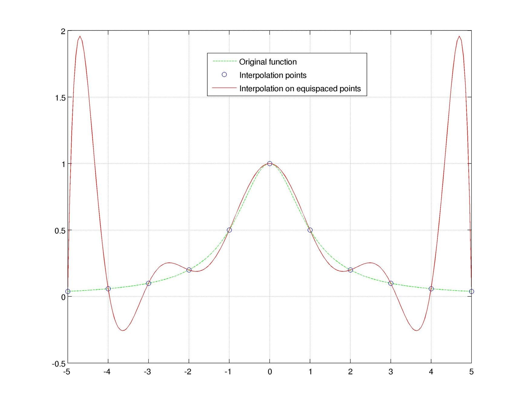
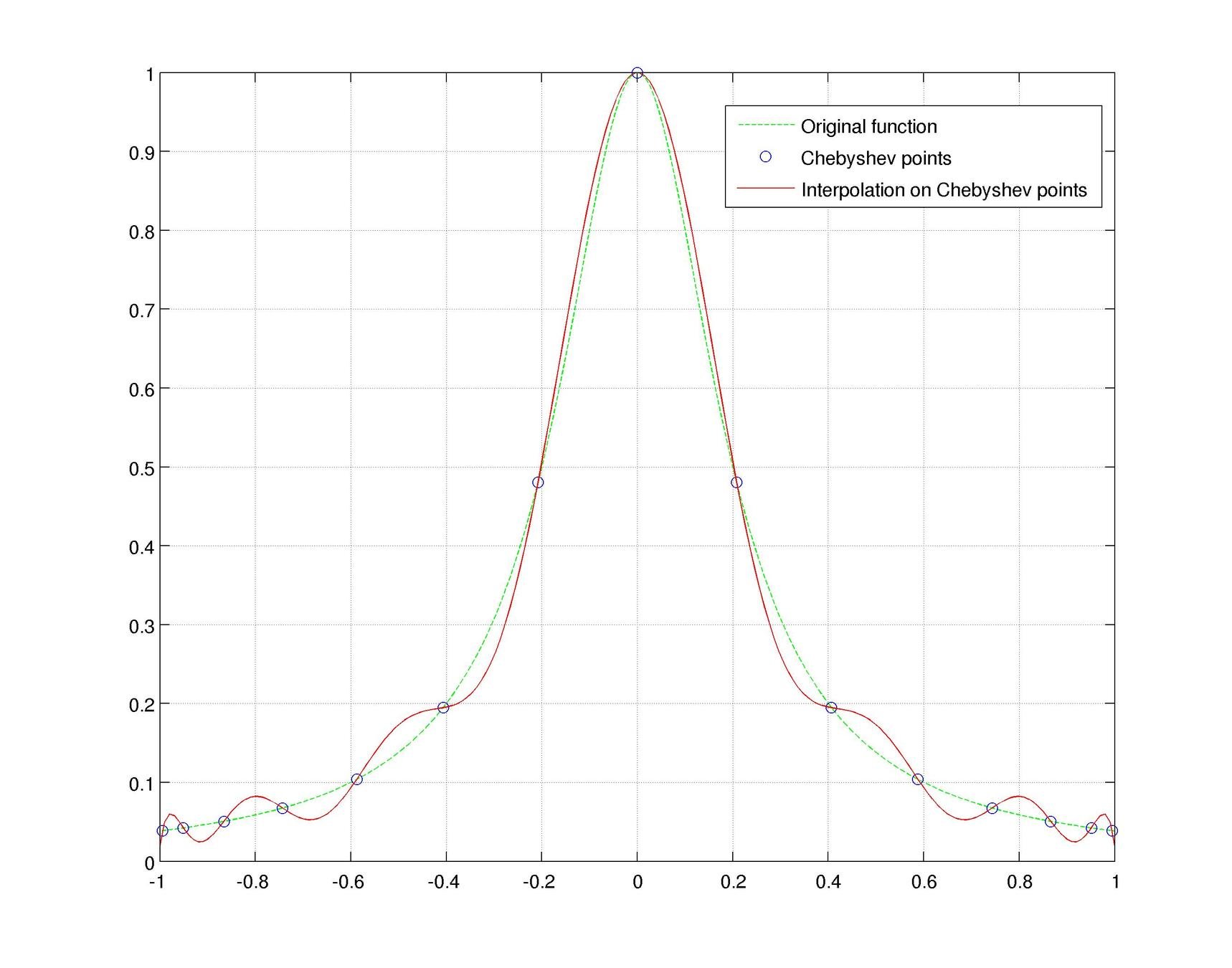
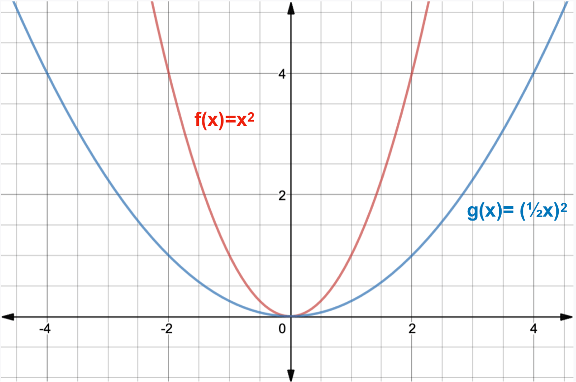
Motivation #1. The Runge effect is taught in every Num. Calculus course. Basically, we avoid it by resampling to Chebyshev or Chebyshev-Lobatto nodes...
what is the take-home message?
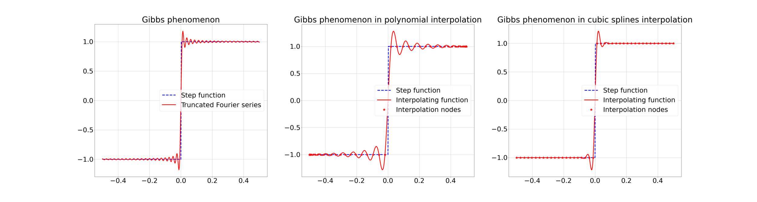
Motivation #2. The Gibbs effect.
Gibbs effect (in a nutshell):
- Appears at discontinuities as oscillatory;
- Does not vanish as \(N\to\infty\);
- As \(N\to\infty\) their frequency grows, the amplitude reaches a plateau.

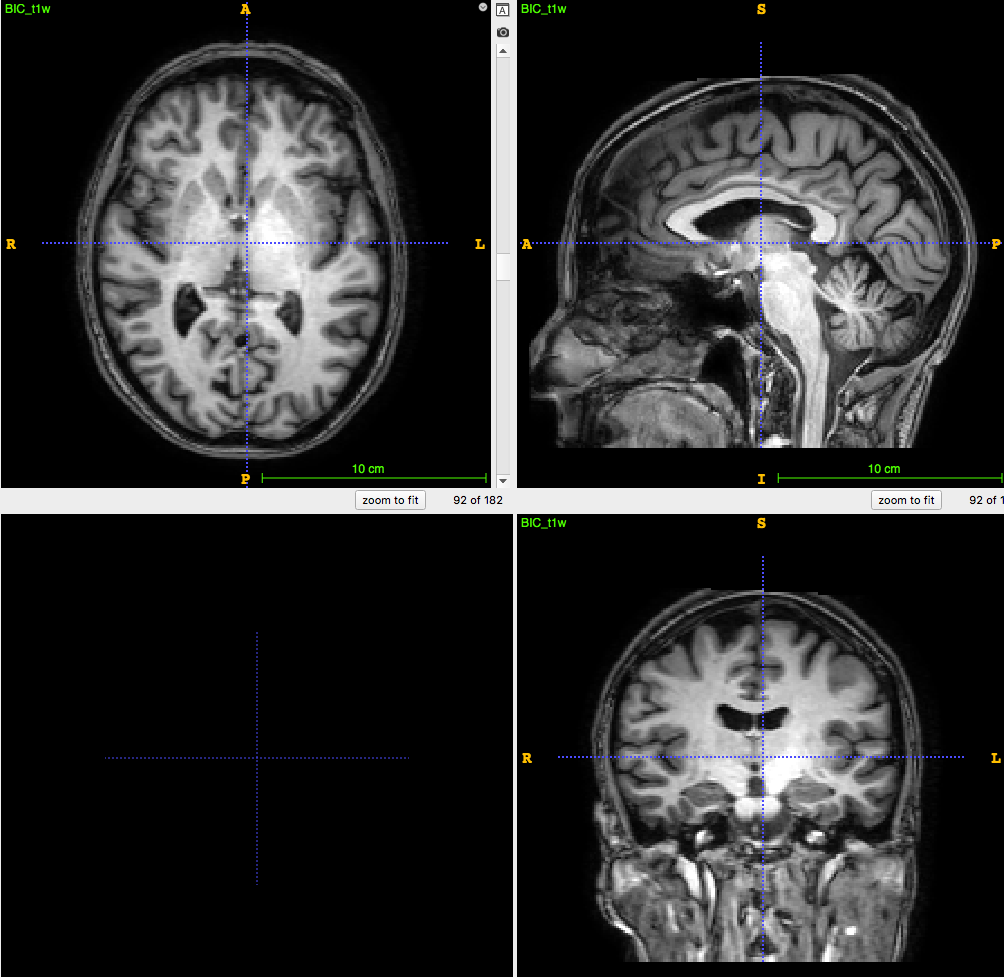
3D T1-weighted MRI:
usually ~1 mm \(^3\) voxel
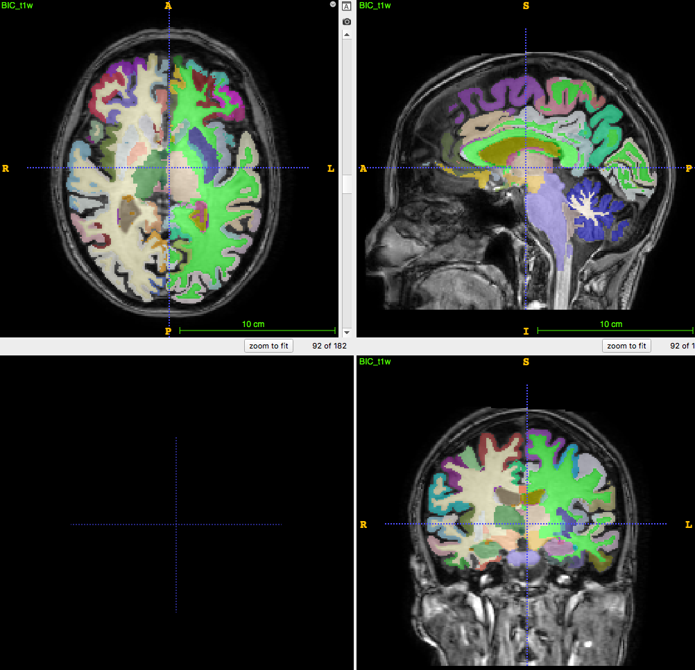
Segmentation/parcellation at full resolution
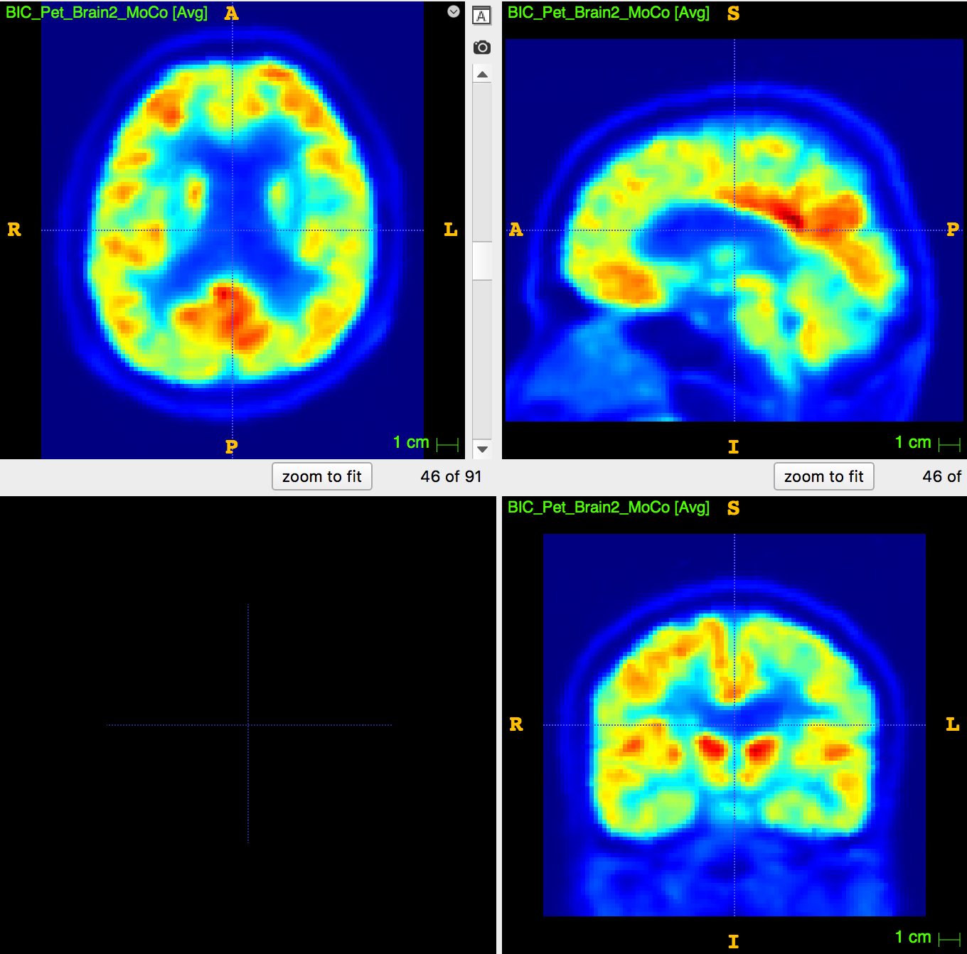
PET image:
usually ~8mm \(^3\) voxel
How to apply segmentation?
1. Undersampling T1 segmentation
2. Upsampling PET image
2. Fake Nodes Approach (FNA)
Interpolation on Fake Nodes, or interpolation via Mapped Bases is a technique that applies to any interpolation method in any dimension. It has shown in many cases the ability of obtaining a better interpolation without getting new samples.
This means that, provided that the original nodes are a sufficient sample of the given signal, it can be possible in principle to provide an interpolation of smaller error.
Given a function
f: \Omega \subseteq \mathbb{R}^d \longrightarrow \mathbb{R}\;\;\;\;\; {d \in \mathbb{N}},
a set of nodes
X = \{ x_0, \dots, x_N \in \Omega \},
and a set of basis functions
\mathcal{B} = \{ b_i: \Omega \longrightarrow \mathbb{R} \}_{i = 0, \ldots, N}
The interpolant is given by a function
\displaystyle \mathcal{P}(\bm{x}) = \sum_{i=0}^{N} c_i b_i(\bm{x})
s.t.
\mathcal{P}(\bm{x}_i)=y_i:=f(\bm{x}_i) \;\;\forall i
\mathcal{B} = \{ b_i \circ S: \Omega \longrightarrow \mathbb{R}^d \}_{i = 0, \ldots, N}
\displaystyle \mathcal{R}^s(\bm{x}) = \sum_{i=0}^{N} c_i b_i(S(\bm{x}))
\mathcal{R}^s(\bm{x}_i)=y_i:=f(\bm{x}_i) \;\;\forall i
FNA is an interpolation over the original basis \(\mathcal{B}\) of a function \(g: S(\Omega) \longrightarrow\mathbb{R}\)
on the fake nodes
\[S(X) = \{S(x_i) \}_{i=0, \dots, N}.\]
\(g\in C^s\) must satisfy \(g(S(x_i)) = f(x_i)\;\;\forall i\).
If \(\mathcal{P} \) is an interpolant on \(g\) on the fake nodes, then \(\mathcal{P}(S(x)) = g(S(x)) \) for all \(x\in X\),
then \(\mathcal{R}^s := \mathcal{P} \circ S\) is an interpolant on \(f\). In fact \(\mathcal{R}^s (x)= \mathcal{P} (S(x)) = f(x) \) for all \(x\in X\).
Common hypothesis from now on:
(1.) The mapping \(S\) is injective \(\longrightarrow\) Fake Nodes do not overlap
(2.) We interpolate a function \(g\) s.t. \( g\circ S =f\). Such function exists as (1.) holds
Proposition 2.1 [Equivalence of the Lebesgue constant]
The Lebesgue constant associated to the mapped nodes \(\Lambda^s(\Omega)\) is so that
\[\Lambda^s(\Omega) = \Lambda(S(\Omega)).\]
This means that the interpolation via mapped basis inherits the Lebesgue constant of the original basis in the Fake Nodes, and (by consequence) the stability.
Lemma 2.1 [Equivalence of a cardinal basis]
If \(\{u_i\}_{i=0,\dots,N}\) is a cardinal basis on the Fake Nodes \(S(X)\) then
\( \{u_i\circ S\}_{i=0,\dots,N}\) is cardinal too on \(X\)
Proposition 2.2 [Stability]
Let \(\mathcal{R}^s_{\tilde{f}}\) be the interpolant of the function values
\(\tilde{f}(x_i)\), \(i=1,\ldots,n\). Then,
\[ \lvert\lvert \mathcal{R}_f^s - \mathcal{R}_{\tilde f}^s \rvert\rvert_{\infty,\Omega} \leq \Lambda^s(\Omega) \; \| f-{\tilde f} \|_{\infty, X_n}.\]
Summing up: suppose that if we know that a basis is more stable over a different distribution of interpolation nodes \(X\), but all we have on our dataset is the samples on some other nodes \(Y\). All we have to do is finding a mapping \(S\) such that \(S(Y) =X\), as regular as possible and apply the FNA with such mapping.
3. Application: Image resampling
A three-dimesional MRI can be ~ \(10^8\) voxels (256x256x256 takes ~800Mb in double precision, uncompressed) and counting. Hence a fast, lightweight interpolation method is needed.
Let us take a \(10^8\) voxels image. The interpolation matrix would be \(10^8 \times 10^8\) .... ~80Pb in double precision!
What is the fastest interpolation method?
- Choose a basis;
- Compute Interpolation/Evaluation matrices;
- Solve a linear system;
- Multiply Eval. matrix by coefficients.
So we need to choose a basis:
- Separable → the interpolation is computed on each axis sequentially;
- Cardinal → no need to compute or invert the Interpolation matrix;
- Compact supported → Evaluation matrix is sparse.
To achieve that we have to suppose that the interpolation nodes are on a equispaced grid.
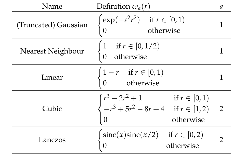
We can choose
\[\mathcal{P}_f (\bm{x}) = \sum_{ijk} f(\bm{x}_{ijk})W_{ijk}(\bm{x})\]
with
\[W_{ijk}(x, y, z) = w(x-x_i)\; w(y-y_i) \;w(z-z_i)\]
the separable basis with \(w(t-t_i)\) a cardinal and compact-supported basis.
This is called interpolation by convolution.
4. Error bounds and Gibbs Effect
Definition 4.1 Let \(f: \Omega \subseteq \mathbb{R}^d \longrightarrow \mathbb{R}\) be a piecewise continuous function. The function \(f\) admits a (local) modulus of continuity
$$\omega_{\bm x_0}(\delta): \mathbb{R}^{+} \longrightarrow \mathbb{R}^{+}$$
in \(\bm x_0\in\Omega\) if
\[ |f(\bm x) - f(\bm x_0) | \leq \omega_{\bm x_0}(\delta) \;\;\forall \bm x \in \Omega \text{ s.t. } \|\bm x- \bm x_0\|\leq \delta, \]
where \(\|\cdot\|\) is an arbitrary norm.
In order to provide an estimate of the interpolation error for the image interpolation by convolution, we need to provide some background theory.
Theorem 4.1 Let \(f\) be a d-variate and bounded function admitting a local modulus of continuity \(\omega_{\bm x} (\delta)\). Let \(\mathcal{P}f\) be its interpolant by convolution. Then, there exits some \(\delta^* > 0\) such that
\[ |\mathcal{P}f (\bm x) - f(\bm x)| \leq \omega_{\bm x} (\delta^*)\,. \]
Corollary 4.1 Let \(f\) be a d-variate and bounded function admitting a global modulus of continuity \(\omega_{\bm x} (\delta)\). Let \(\mathcal{P}f\) be its interpolant by convolution. Then, there exitsdome \(\delta^* > 0\) such that
\[ |\mathcal{P}f (\bm x) - f(\bm x)| \leq \omega (\delta^*)\,. \]
Lemma 4.1 A d-variate, Lipschitz-continuous function \(f\) admits a modulus of continuity of the form
\[\omega(\delta) = K\delta \]
being \(K\) the Lipschitz constant.
Lemma 4.2 A piecewise d-variate, Lipschitz-continuous function $f$ admits a modulus of continuity of the form
\[\omega(\delta) = K\delta + D \]
5. Experiments
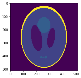
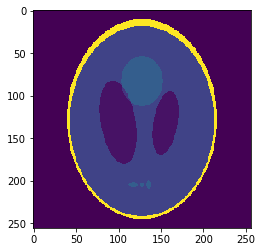
In silico validation: the Shepp-Logan 3D phantom
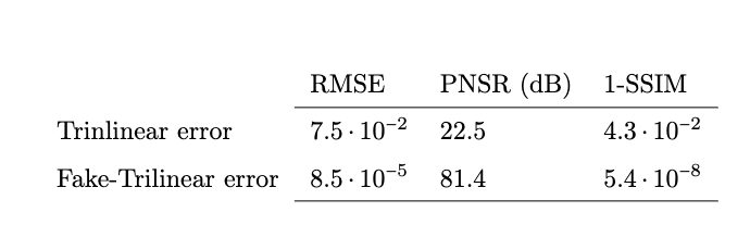
Using a phantom the gold standard is known and we can analyse the errors of approximation.
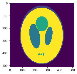
High resolution "morphological" image
Segmentation mask
Low resolution "functional" image
1mm^3
8mm^3
1mm^3
\((2mm)^3\)
\(1mm^3\)
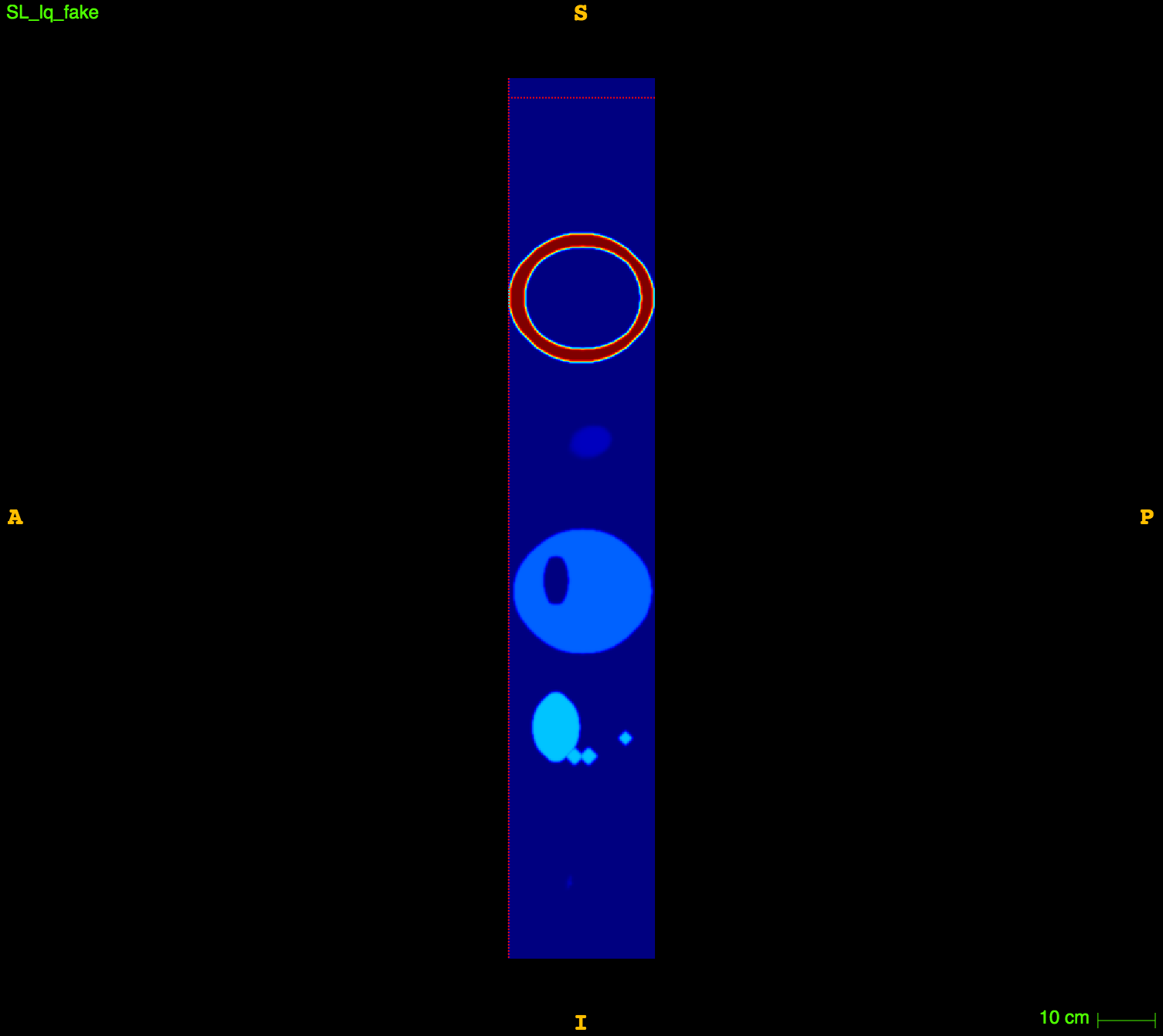
Fake image
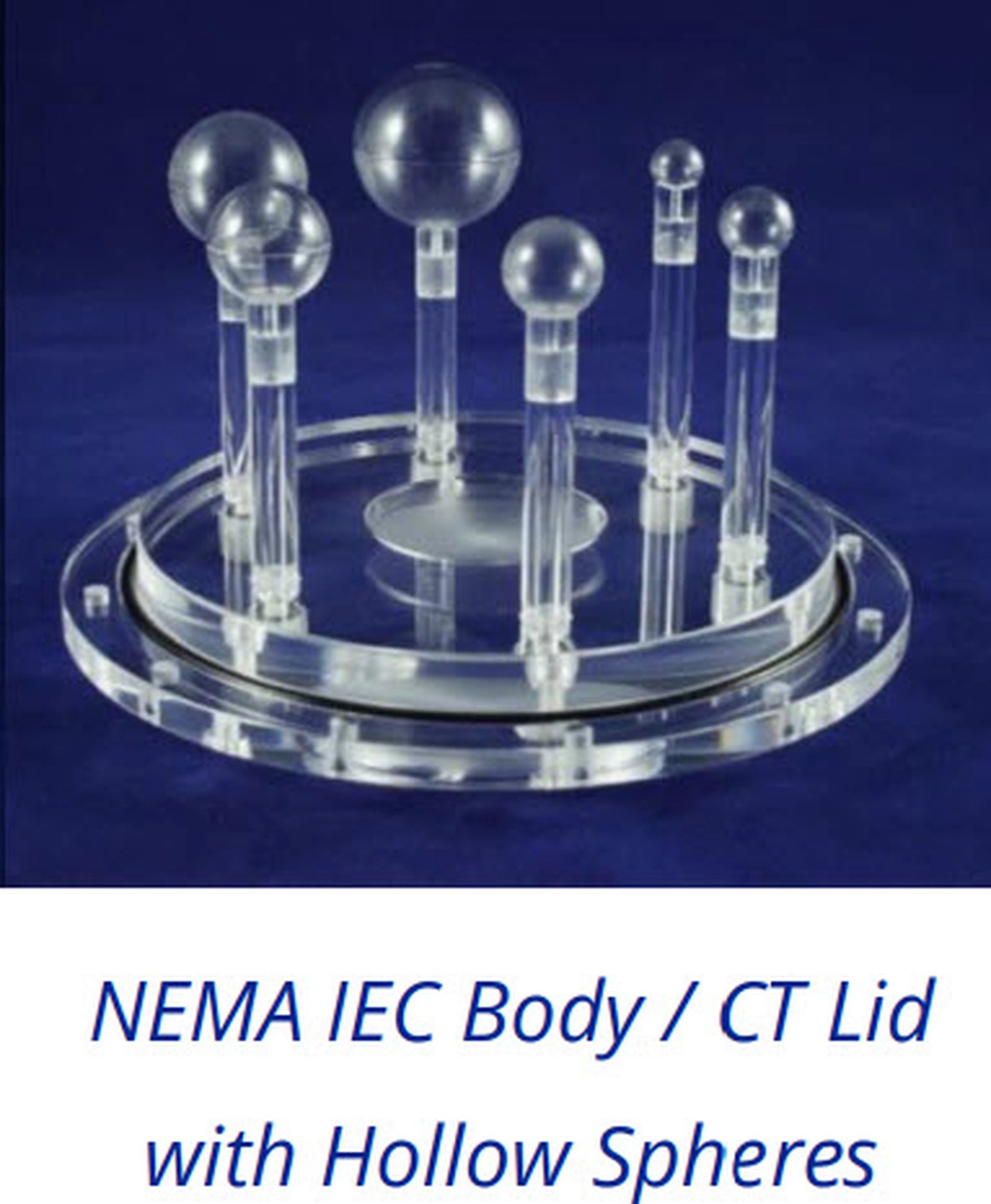
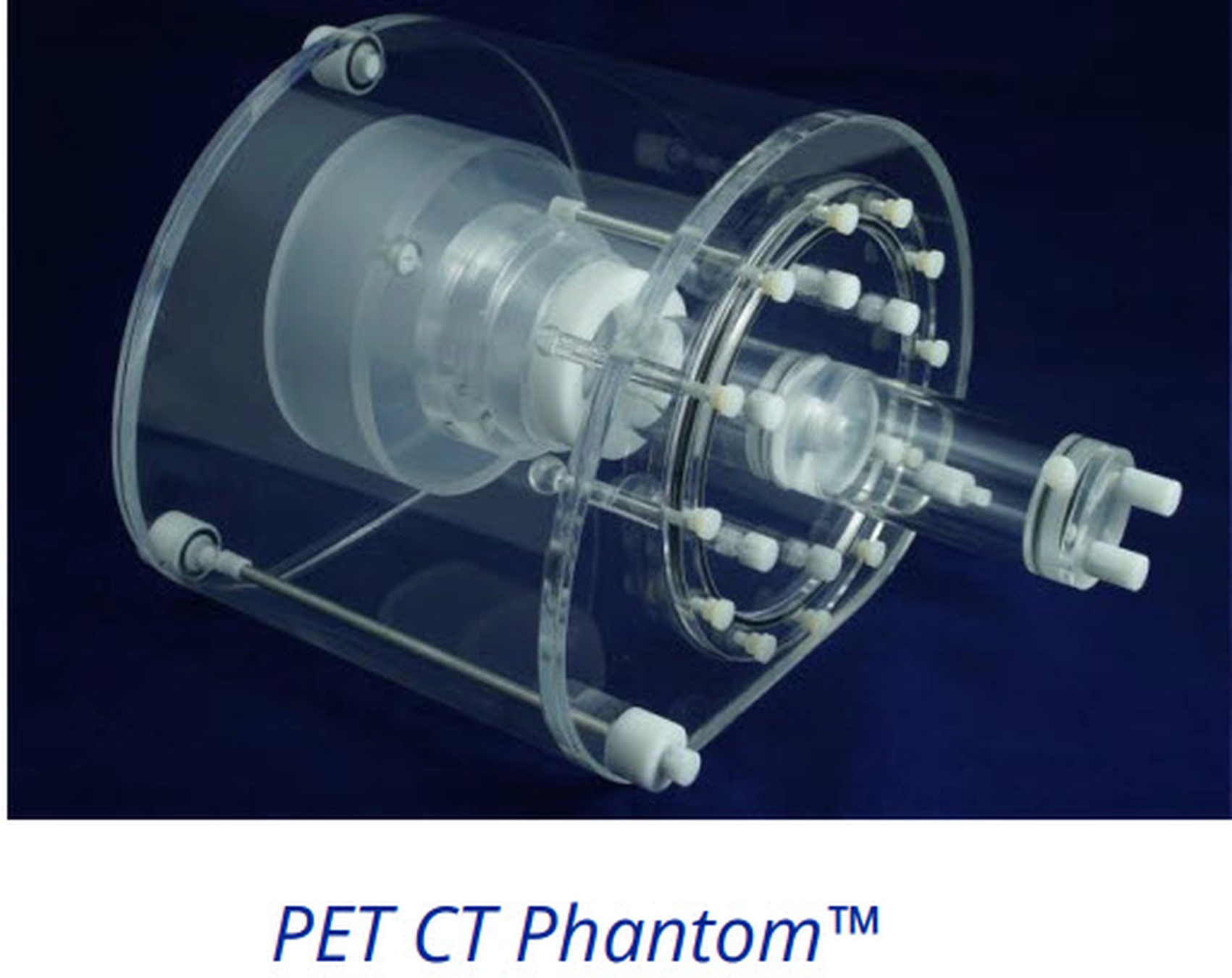
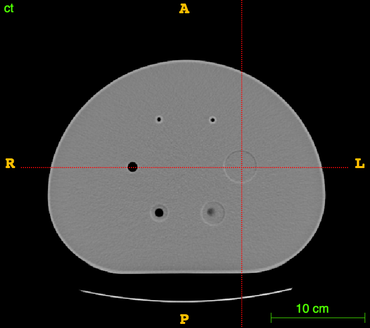
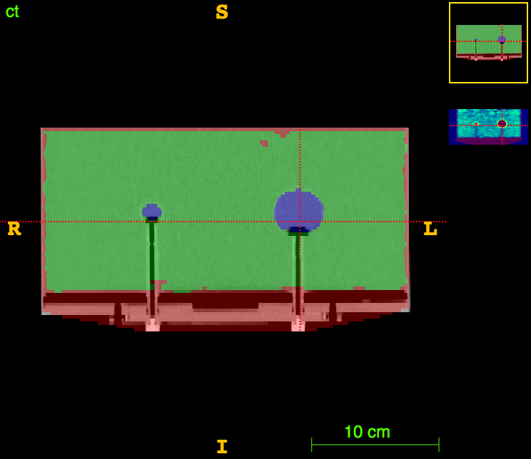
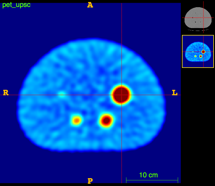
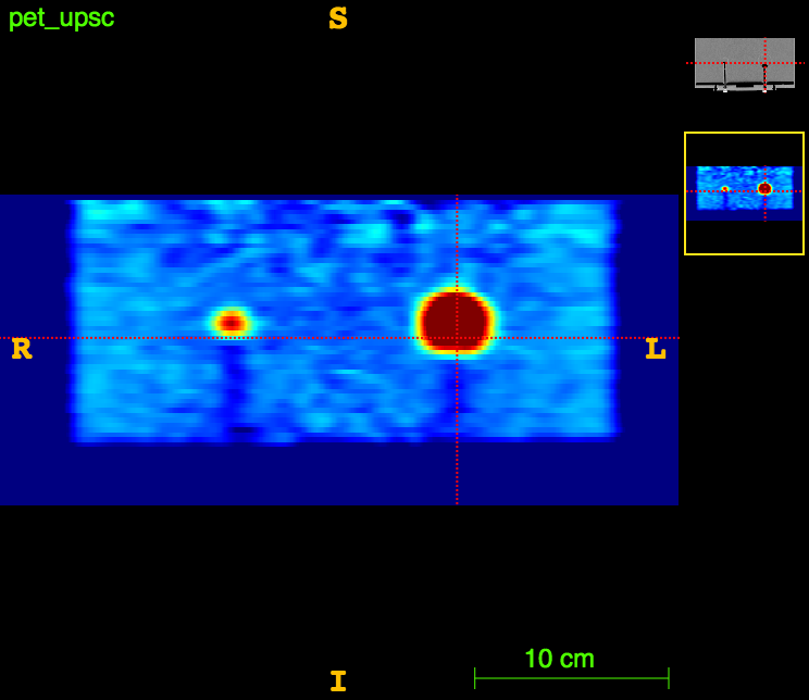
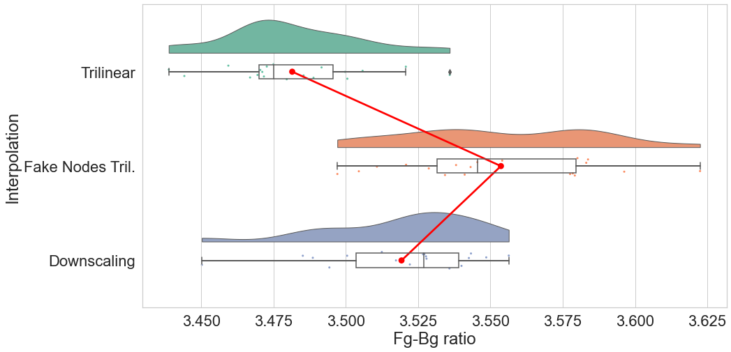
In vitro validation:
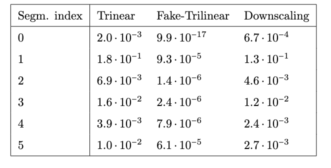
The RIDER PET/CT phantom images is a dataset of repeated scans of a dummy (20 scans of the same phantom).
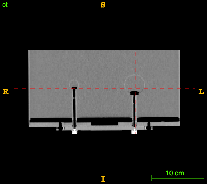
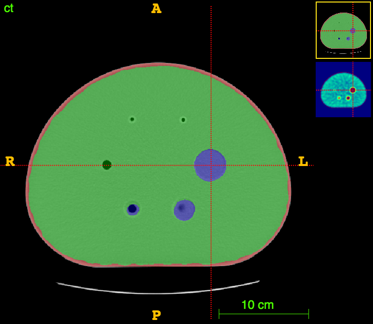
Axial
Sagittal
CT
Axial
Axial
CT
CT segm.
PET
6. Conclusions
- We have defined the FNA as a powerful instrument to cheat on the nodes;
- applications in imaging have been studied;
- we have proven the presence of Gibbs effect in image oversampling;
- we have proposed a Fake-Nodes based workaround in the context of Multimodal medical imaging;
- we have evaluated such method both in silico and in vitro.
[1] Burger, W.; Burge, M.J., Principles of digital image processing: core algorithms; Springer, 2009.
[2] Dumitrescu.; Boiangiu. A Study of Image Upsampling and Downsampling Filters. Computers doi:10.3390/computers8020030.4139
[3] S. De Marchi, F. Marchetti, E. Perracchione, Jumping with Variably Scaled Discontinuous Kernels (VSDKs), BIT Numerical Mathematics 2019.
[4] S. De Marchi, F. Marchetti, E. Perracchione, D. Poggiali, Polynomial interpolation via mapped bases without resampling, JCAM 2020.
[5] S. De Marchi, F. Marchetti, E. Perracchione, D. Poggiali, Multivariate approximation at Fake Nodes, AMC 2021.
[5] S. De Marchi, G. Elefante, E. Perracchione, D. Poggiali, Quadrature at Fake Nodes, DRNA 2021.
[6] D. Poggiali, D. Cecchin, C. Campi, S. De Marchi, Oversampling errors in multimodal medical imaging are due to the Gibbs effect, Mathematics 2021.
[7] D. Poggiali, D. Cecchin, S. De Marchi, Reducing the Gibbs effect in multimodal medical imaging by the Fake Nodes Approach, JCMDS 2022.
[8] C. Runge, Uber empirische Funktionen und die Interpolation zwischen aquidistanten Ordinaten, Zeit. Math. Phys, 1901.
Thanks for your attention!
Multivariate Fake Nodes Approach
By davide poggiali


