Image analysis
introduction
01
Images and data
How images are created and stored
Image visualization
Opening and visualizing your data with ImageJ
Simple measurements
How to manually explore and measure your data
Images and data
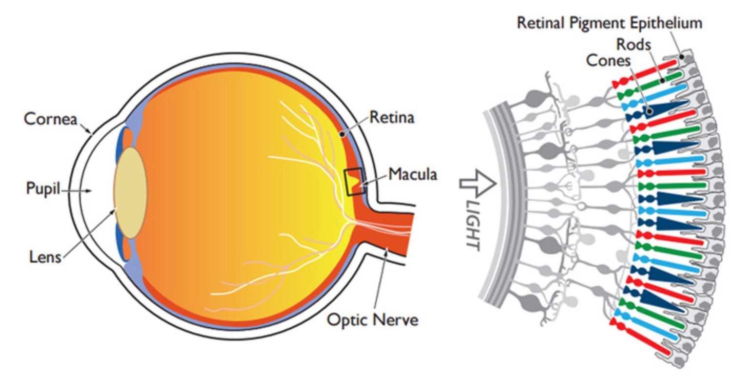
sample


radiation
camera
sensor
digital signal

continuous signal
discrete signal
dark
bright
1bit
(2 levels)
2bit
(4 levels)
3bit
(8 levels)
0
1
00
01
10
11
000
001
011
010
100
101
110
111
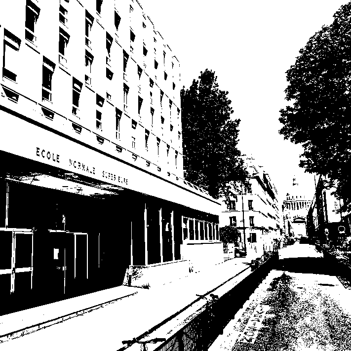
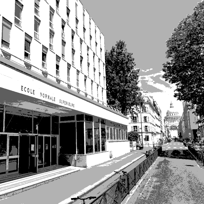
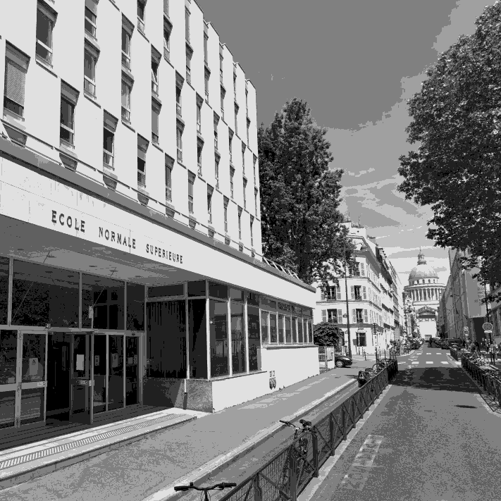
1bit
2bit
3bit
8bit

16bit
256 levels
65 536 levels


32bit images are a little special, they use floating point precision
- Max value: 3x10^38
- Allows positives or negatives
- Allows decimal values
This means using 32bits is interesting when performing mathematical operations!
File size increases together with bit-depth
512x512 pixels image:
8bit = 256 KB
16bit = 512 KB
32bit = 1024 KB (1 MB)
ATTENTION
You can scale down, but never scale up!
What about color images?

additive color model

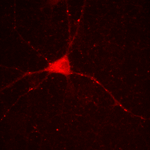
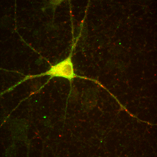
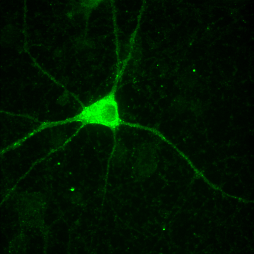
+
=


red channel
green channel
composite image
but remember:
the colors we see in microscopy images are purely arbitrary!
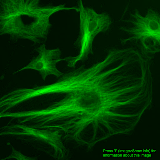
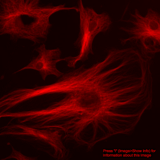
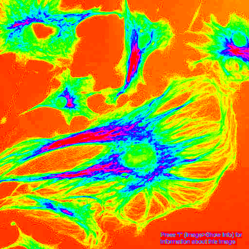


0
255
0
255
0
255
real size and pixel size
- Objective magnification
- Lens magnification
(in some microscopes, it is possible to get extra mag of 1.25x, 1.6x or 2x) - C mount (is usually 1x)
- Pixel size – is the actual pixel size of the camera that is attached to the microscope.
- Binning – i.e. combining a cluster of pixels to a single pixel.
The common options are 1X1, 2X2 and 4X4.
The pixel size depends on optical and camera settings
Laser scanning techniques don't have a fixed physical pixel size
Although a minimum size is always restrained by the diffraction limit of light
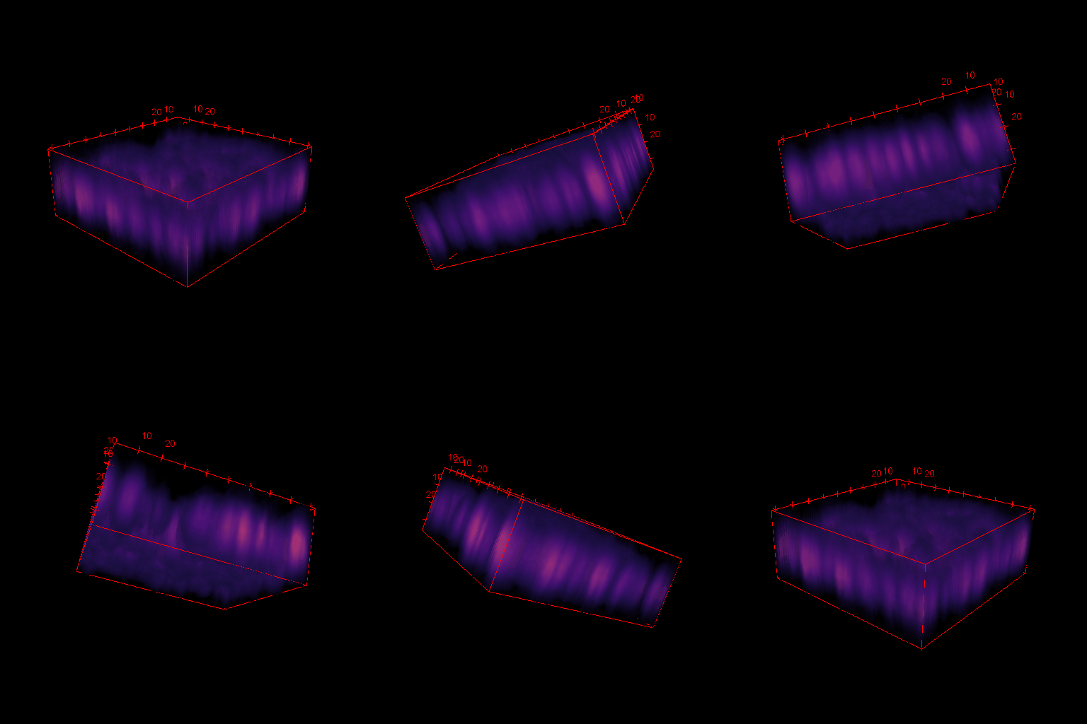
3D images in microscopy

X
Y
depth
(Z)


X
Y
Z step
}
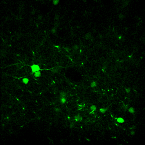
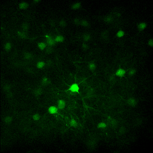
X and Y resolution is usually much higher than axial (Z) resolution!
Your biggest enemy when making 3D acquisitions is the PSF!
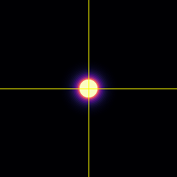
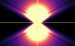
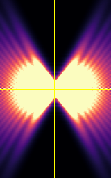
XY
YZ
XZ
Point-spread-function (PSF)
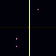


XY
YZ
XZ
Spherical beads with 200nm
Image visualization
For opening images of different formats, bio-formats is a great choice

- Open Fiji
- Load a simple 2D image (synapses.tif)
- Basic commands: zoom and pan
- Change colormaps (attention perceptually uniform colormaps)
- Understand a histogram (Analyse > Histogram)
- Adjust brightness and contrast
- Duplicate image, and duplicate a crop region
PRACTICAL EXERCISE
01
- Load a 3D image (embryo.tif)
- Notice the slider for the Z dimension
- Adjust brightness and colormap (explore Auto, Reset and Set options)
- Make a Z projection (Image > Stacks > Z project)
- Explore the Orthogonal views (Image > Stacks > Orthogonal Views)
- Test the volume 3D Viewer (understand threshold and transparency)
- Apply Process > Subtract background (radius 20) and run 3D viewer again
- Change background color and record a rotation movie
PRACTICAL EXERCISE
02
- Load a 3D+time image (drosophila_brain.tif)
- Adjust brightness and contrast
- Use orthogonal views to understand the movement
- Check Image > Properties
- Make a Z Max projection
- Select font properties (Edit > Options > Fonts)
- Convert Image to RGB (Image > Type > RGB color)
- Insert a frame label (Image > Stacks > Label)
- Export video (File > Save as > AVI)
- Remove overlay (Image > Overlay > Remove overlay)
PRACTICAL EXERCISE
03
- Load a multi-channel image (5channels.tif)
- Make a Z max projection, reset brightness and contrast
- Open the channels tool (Image >Color > Channels tool)
- Understand the difference between Composite and Color
- Split channels (Image > Color > Split channels)
- Merge only channels 1 and 3 (Image > Color > Merge channels)
- Set C1 as magenta, C2 as green
- Understand that brightness and contrast is channel independent
PRACTICAL EXERCISE
04
Simple measurements
05
PRACTICAL EXERCISE
- Load again the synapses image (synapses.tif)
- Choose the measurements (Analyse > Set Measurements)
- Select Area, Mean gray value and Integrated density
- Zoom in into one synapse, and make a circle around it
- Go to Analyse > Measure (or press Ctrl+M)
- Move your circle to another synapse, and press Ctrl+M again
- Save your Results table (File > Save As from the table window)
06
PRACTICAL EXERCISE
- Clear all your measurements
- Make a line crossing one synapse
- Select Analyse > Plot profile
- Click Live and change your selection line
- Make a line that cross a synapse, and select Data > Add Fit
- Select Gaussian Fit and press OK
07
PRACTICAL EXERCISE
- Clear all your measurements
- Make a square crossing one synapse
- Select Analyse > Surface plot
- Select Draw Wireframe, Draw Axis and Smooth and click OK
image_analysis@list01.biologie.ens.fr
ImageAnalysisTutorials01
By Felipe Delestro
ImageAnalysisTutorials01
- 830


