Data Cleaning 資料清理
陳達泓 Denny
denny20700@gmail.com
2019.12.02
使用tidyr整理資料

資料分析流程:
Let's Go!

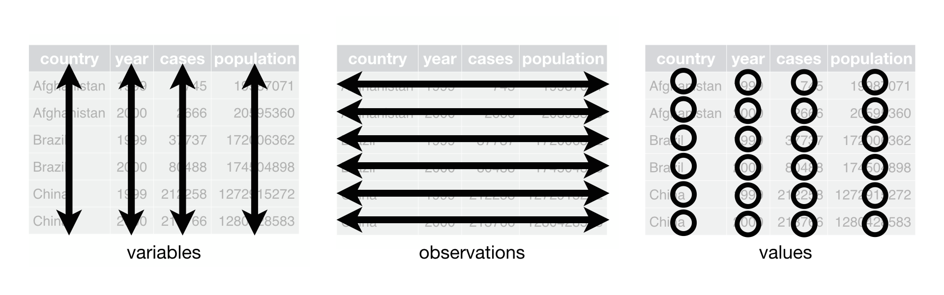
什麼是整齊的資料 tidy data ?

1. 每個變數(variable)都必須要有自己的資料欄
2. 每個觀察(observation)都必須要有自己的資料列
3. 每個值(value)都必須要有自己的資料格
這次我們首先會用到 gather 以及 spread
#呼叫
library(tidyr) ; # require(tidyr)
#他也同時是tidyverse這個套件的一員,我們呼叫tidyverse就好
library(tidyverse)
在未呼叫套件時使用函式
#指定套件呼叫函式
tidyr::gather() ; tidyr::spread()
1. 找出變數與觀察值在哪裡

2. 解決兩個常見的問題之一:
-
一個變數有可能分散到多個資料欄 -
一個觀察有可能散布在多個資料列
猜猜哪一個要用到gather and spread
Answer click me
大家可以先在 RStudio 上面輸入
🔻
cat("table1  \n") ; table1
cat("table2  \n") ; table2
cat("table3  \n") ; table3
cat("table4a \n") ; table4a
cat("table4b \n") ; table4b
cat("table5  \n") ; table5
> cat("table1 \n") ; table1
table1
# A tibble: 6 x 4
country year cases population
<chr> <int> <int> <int>
1 Afghanistan 1999 745 19987071
2 Afghanistan 2000 2666 20595360
3 Brazil 1999 37737 172006362
4 Brazil 2000 80488 174504898
5 China 1999 212258 1272915272
6 China 2000 213766 1280428583
> cat("table2 \n") ; table2
table2
# A tibble: 12 x 4
country year type count
<chr> <int> <chr> <int>
1 Afghanistan 1999 cases 745
2 Afghanistan 1999 population 19987071
3 Afghanistan 2000 cases 2666
4 Afghanistan 2000 population 20595360
5 Brazil 1999 cases 37737
6 Brazil 1999 population 172006362
7 Brazil 2000 cases 80488
8 Brazil 2000 population 174504898
9 China 1999 cases 212258
10 China 1999 population 1272915272
11 China 2000 cases 213766
12 China 2000 population 1280428583
> cat("table3 \n") ; table3
table3
# A tibble: 6 x 3
country year rate
* <chr> <int> <chr>
1 Afghanistan 1999 745/19987071
2 Afghanistan 2000 2666/20595360
3 Brazil 1999 37737/172006362
4 Brazil 2000 80488/174504898
5 China 1999 212258/1272915272
6 China 2000 213766/1280428583
> cat("table4a \n"); table4a
table4a
# A tibble: 3 x 3
country `1999` `2000`
* <chr> <int> <int>
1 Afghanistan 745 2666
2 Brazil 37737 80488
3 China 212258 213766
> cat("table4b \n"); table4b
table4b
# A tibble: 3 x 3
country `1999` `2000`
* <chr> <int> <int>
1 Afghanistan 19987071 20595360
2 Brazil 172006362 174504898
3 China 1272915272 1280428583
> cat("table5 \n") ; table5
table5
# A tibble: 6 x 4
country century year rate
* <chr> <chr> <chr> <chr>
1 Afghanistan 19 99 745/19987071
2 Afghanistan 20 00 2666/20595360
3 Brazil 19 99 37737/172006362
4 Brazil 20 00 80488/174504898
5 China 19 99 212258/1272915272
6 China 20 00 213766/1280428583Gathering 聚集
寬資料轉長資料
tidyr::gather()
Usage
gather(data, key = "key", value = "value", ..., na.rm = FALSE,
  convert = FALSE, factor_key = FALSE)
Argument
key. value : Names of new key and value columns, as strings or symbols.
key:就是你想把原本是colnames的變成values的那一欄名稱
value:原本column對應的值所產生的新欄位名稱
key
value
table4a
# A tibble: 3 x 3
  country     `1999` `2000`
* <chr>        <int>  <int>
1 Afghanistan    745   2666
2 Brazil       37737  80488
3 China       212258 213766

tidyr::gather()
Usage
gather(data, key = "key", value = "value", ..., na.rm = FALSE,
  convert = FALSE, factor_key = FALSE)
gather(table4a, `1999`, `2000`, key = "Year", value = "cases")
gather(table4a, "key", "value", -country)
# A tibble: 6 x 3
country Year cases
<chr> <chr> <int>
1 Afghanistan 1999 745
2 Brazil 1999 37737
3 China 1999 212258
4 Afghanistan 2000 2666
5 Brazil 2000 80488
6 China 2000 213766
key:就是你想把原本是colnames的變成values的那一欄名稱
value:原本column對應的值所產生的新欄位名稱
table4a
# A tibble: 3 x 3
  country     `1999` `2000`
* <chr>        <int>  <int>
1 Afghanistan    745   2666
2 Brazil       37737  80488
3 China       212258 213766
Spreading 分散
長資料轉寬資料
tidyr::spread()
Usage
spread(data, key, value, fill = NA, convert = FALSE, drop = TRUE, sep = NULL)
Argument key. value : Column names or positions. This is passed to tidyselect::vars_pull().
key: 含有應該要是變數名稱的資料欄
value: 來自多個變數的值的資料欄
> table2
# A tibble: 12 x 4
   country      year type            count
   <chr>       <int> <chr>           <int>
 1 Afghanistan  1999 cases             745
 2 Afghanistan  1999 population   19987071
 3 Afghanistan  2000 cases            2666
 4 Afghanistan  2000 population   20595360
 5 Brazil       1999 cases           37737
 6 Brazil       1999 population  172006362
 7 Brazil       2000 cases           80488
 8 Brazil       2000 population  174504898
 9 China        1999 cases          212258
10 China        1999 population 1272915272
11 China        2000 cases          213766
12 China        2000 population 1280428583
key
value
tidyr::spread()
Usage
spread(data, key, value, fill = NA, convert = FALSE, drop = TRUE, sep = NULL)
key: 含有應該要是變數名稱的資料欄
value: 來自多個變數的值的資料欄
> table2
# A tibble: 12 x 4
   country      year type            count
   <chr>       <int> <chr>           <int>
 1 Afghanistan  1999 cases             745
 2 Afghanistan  1999 population   19987071
 3 Afghanistan  2000 cases            2666
 4 Afghanistan  2000 population   20595360
 5 Brazil       1999 cases           37737
 6 Brazil       1999 population  172006362
 7 Brazil       2000 cases           80488
 8 Brazil       2000 population  174504898
 9 China        1999 cases          212258
10 China        1999 population 1272915272
11 China        2000 cases          213766
12 China        2000 population 1280428583
spread(table2, key = type, value = count)# A tibble: 6 x 4
country year cases population
<chr> <int> <int> <int>
1 Afghanistan 1999 745 19987071
2 Afghanistan 2000 2666 20595360
3 Brazil 1999 37737 172006362
4 Brazil 2000 80488 174504898
5 China 1999 212258 1272915272
6 China 2000 213766 1280428583
Exercises
people <- tribble(
  ~name,              ~key,      ~value,
  "Phillip Woods",    "age",     45,
  "Phillip Woods",    "height",  185,
  "Phillip Woods",    "age",     50,
  "Jessica Cordero",  "age",     37,
  "Jessica Cordero",  "height",  156,
)
這個tibble應該要gather 還是 spread?
有沒有辦法執行? why? 怎麼解決?
Solutions
1
people %>% group_by(name) %>%
 distinct(key, .keep_all = T) %>%
  spread(key, value)
# A tibble: 2 x 3
# Groups: name [2]
name age height
<chr> <dbl> <dbl>
1 Jessica Cordero 37 156
2 Phillip Woods 45 185
drop duplicated or create a new column
Tips
people %>% group_by(name, key) %>%
  mutate(obs = row_number()) %>%
  spread(key, value)
# A tibble: 3 x 4
# Groups: name [2]
name obs age height
<chr> <int> <dbl> <dbl>
1 Jessica Cordero 1 37 156
2 Phillip Woods 1 45 185
3 Phillip Woods 2 50 NA
2
Exercises
preg <- tribble(
  ~pregnant, ~male, ~female,
  "yes", NA, 10,
  "no", 20, 12
)
這個tibble應該要gather 還是 spread?
Solutions
gather(preg,male, female, key = "sex", value = "count")# A tibble: 4 x 3
pregnant sex count
<chr> <chr> <dbl>
1 yes male NA
2 no male 20
3 yes female 10
4 no female 12
我們完成處理 table2 & table4 了!
但還有 table3。
table3 有什麼問題呢?
: 其中一個資料欄 (rate) 含有兩個變數(case & population)
table3
# A tibble: 6 x 3
  country      year rate
* <chr>       <int> <chr>
1 Afghanistan  1999 745/19987071
2 Afghanistan  2000 2666/20595360
3 Brazil       1999 37737/172006362
4 Brazil       2000 80488/174504898
5 China        1999 212258/1272915272
6 China        2000 213766/1280428583
case / population
這次我們首先會用到 separate 以及 unite
Separate 分離
一個資料欄拆成多個資料欄
Usage
separate(data, col, into, sep = "[^[:alnum:]]+", remove = TRUE, convert = FALSE, extra = "warn", fill = "warn", ...)
table3 %>% separate(col = rate, into = c("cases", "population"))
table3 %>% separate(rate, into = c("cases", "population"), sep = "/")
# A tibble: 6 x 4
country year cases population
<chr> <int> <chr> <chr>
1 Afghanistan 1999 745 19987071
2 Afghanistan 2000 2666 20595360
3 Brazil 1999 37737 172006362
4 Brazil 2000 80488 174504898
5 China 1999 212258 1272915272
6 China 2000 213766 1280428583
table3
# A tibble: 6 x 3
  country      year rate
* <chr>       <int> <chr>
1 Afghanistan  1999 745/19987071
2 Afghanistan  2000 2666/20595360
3 Brazil       1999 37737/172006362
4 Brazil       2000 80488/174504898
5 China        1999 212258/1272915272
6 China        2000 213766/1280428583
tidyr::separate()
tidyr::separate()
Usage
separate(data, col, into, sep = "[^[:alnum:]]+", remove = TRUE, convert = FALSE, extra = "warn", fill = "warn", ...)
table3 %>% separate(year, into = c("century", "year"), sep = 2)table3
# A tibble: 6 x 3
country year rate
* <chr> <int> <chr>
1 Afghanistan 1999 745/19987071
2 Afghanistan 2000 2666/20595360
3 Brazil 1999 37737/172006362
4 Brazil 2000 80488/174504898
5 China 1999 212258/1272915272
6 China 2000 213766/1280428583
# A tibble: 6 x 4
  country     century year  rate
  <chr>       <chr>   <chr> <chr>
1 Afghanistan 19      99    745/19987071
2 Afghanistan 20      00    2666/20595360
3 Brazil      19      99    37737/172006362
4 Brazil      20      00    80488/174504898
5 China       19      99    212258/1272915272
6 China       20      00    213766/1280428583
Unite 合併
多個資料欄合成一個資料欄
tidyr::unite()
Usage
unite(data, col, ..., sep = "_", remove = TRUE)
Argument
col The name of the new column, as a string or symbol.
... A selection of columns. If empty, all variables are selected.
table5 %>% unite(new, century, year)# A tibble: 6 x 4
country century year rate
<chr> <chr> <chr> <chr>
1 Afghanistan 19 99 745/19987071
2 Afghanistan 20 00 2666/20595360
3 Brazil 19 99 37737/172006362
4 Brazil 20 00 80488/174504898
5 China 19 99 212258/1272915272
6 China 20 00 213766/1280428583
# A tibble: 6 x 3
  country     new   rate
  <chr>       <chr> <chr>
1 Afghanistan 19_99 745/19987071
2 Afghanistan 20_00 2666/20595360
3 Brazil      19_99 37737/172006362
4 Brazil      20_00 80488/174504898
5 China       19_99 212258/1272915272
6 China       20_00 213766/1280428583
tidyr::unite()
Usage
unite(data, col, ..., sep = "_", remove = TRUE)
Argument
col The name of the new column, as a string or symbol.
... A selection of columns. If empty, all variables are selected.
table5 %>% unite(new, century, year, sep = "")# A tibble: 6 x 4
country century year rate
<chr> <chr> <chr> <chr>
1 Afghanistan 19 99 745/19987071
2 Afghanistan 20 00 2666/20595360
3 Brazil 19 99 37737/172006362
4 Brazil 20 00 80488/174504898
5 China 19 99 212258/1272915272
6 China 20 00 213766/1280428583
# A tibble: 6 x 3
  country     new   rate
  <chr>       <chr> <chr>
1 Afghanistan 1999  745/19987071
2 Afghanistan 2000  2666/20595360
3 Brazil      1999  37737/172006362
4 Brazil      2000  80488/174504898
5 China       1999  212258/1272915272
6 China       2000  213766/1280428583
Missing Value 遺失值
Missing Value
一個值有兩種缺失方式 :
1. 明確的: 以NA標示
2. 隱含的: 沒有出現在資資料中
stocks <- tibble(
  year  = c(rep(2015,4), rep(2016, 3)),
  qtr = c(1:4, 1:3),
  return = c(1.88, 0.59, 0.35, NA, 0.92, 0.17, 2.66)
)

stocks %>% spread(year, return)
stocks %>% spread(year, return) %>%
  gather(`2015`, `2016`, key = year, value = return)
stocks %>% spread(year, return) %>%
  gather(`2015`, `2016`, key = year, value = return, na.rm = T)
stocks %>% complete(year, qtr)

treatment <- tribble(
  ~ person,           ~treatment, ~response,
  "Derrick Whitmore", 1,          7,
  NA,                 2,          10,
  NA,                 3,          9,
  "Katherine Burke",  1,          4
)
treatment %>% fill(person)
na.rm : NA remove
complete() : 接受一組資料欄,並會找出所有獨特的組合,然後它會確保原本的資料集中含有所有的那些值,並在必要時填入NA。
fill():他接受一組資料欄,其中妳想要以最近的非缺失值來取代遺失值(上一個觀測值取代)
補充:
spread 裡面的 fill 引數是指想要將NA填補為什麼
使用dplyr的關聯式資料
關連式資料 relational data ?
資料分析很少會涉及單一個資料表,通常你會有很多資料表,而我們必須挑選需要的欄位進行分析。

整體而言,多個資料表被稱為關聯式資料,因為重要的是在資料表之間的關聯。
Mutating joins(變動結合) & Filtering joins(過濾結合)
•inner_join
•left_join
•right_join
•full_join
•semi_join
•anti_join
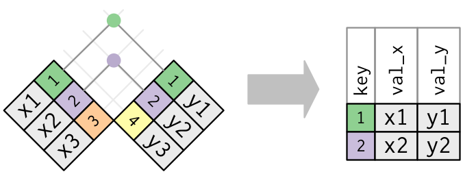
Key 鍵值 : 連接每個資料表的變數
install.packages("nycflights13")
library(nycflights13)

cat("airlines \n") ; airlines
cat("airports \n") ; airports
cat("planes \n") ; planes
cat("weather \n") ; weather
cat("flights \n") ; flights
> cat("airlines \n") ; airlines
airlines
# A tibble: 16 x 2
carrier name
<chr> <chr>
1 9E Endeavor Air Inc.
2 AA American Airlines Inc.
3 AS Alaska Airlines Inc.
4 B6 JetBlue Airways
5 DL Delta Air Lines Inc.
6 EV ExpressJet Airlines Inc.
7 F9 Frontier Airlines Inc.
8 FL AirTran Airways Corporation
9 HA Hawaiian Airlines Inc.
10 MQ Envoy Air
11 OO SkyWest Airlines Inc.
12 UA United Air Lines Inc.
13 US US Airways Inc.
14 VX Virgin America
15 WN Southwest Airlines Co.
16 YV Mesa Airlines Inc.
> cat("airports \n") ; airports
airports
# A tibble: 1,458 x 8
faa name lat lon alt tz dst tzone
<chr> <chr> <dbl> <dbl> <dbl> <dbl> <chr> <chr>
1 04G Lansdowne Airport 41.1 -80.6 1044 -5 A America/New_York
2 06A Moton Field Municipal Airport 32.5 -85.7 264 -6 A America/Chicago
3 06C Schaumburg Regional 42.0 -88.1 801 -6 A America/Chicago
4 06N Randall Airport 41.4 -74.4 523 -5 A America/New_York
5 09J Jekyll Island Airport 31.1 -81.4 11 -5 A America/New_York
6 0A9 Elizabethton Municipal Airport 36.4 -82.2 1593 -5 A America/New_York
7 0G6 Williams County Airport 41.5 -84.5 730 -5 A America/New_York
8 0G7 Finger Lakes Regional Airport 42.9 -76.8 492 -5 A America/New_York
9 0P2 Shoestring Aviation Airfield 39.8 -76.6 1000 -5 U America/New_York
10 0S9 Jefferson County Intl 48.1 -123. 108 -8 A America/Los_Angeles
# ... with 1,448 more rows
> cat("planes \n") ; planes
planes
# A tibble: 3,322 x 9
tailnum year type manufacturer model engines seats speed engine
<chr> <int> <chr> <chr> <chr> <int> <int> <int> <chr>
1 N10156 2004 Fixed wing multi engine EMBRAER EMB-145XR 2 55 NA Turbo-fan
2 N102UW 1998 Fixed wing multi engine AIRBUS INDUSTRIE A320-214 2 182 NA Turbo-fan
3 N103US 1999 Fixed wing multi engine AIRBUS INDUSTRIE A320-214 2 182 NA Turbo-fan
4 N104UW 1999 Fixed wing multi engine AIRBUS INDUSTRIE A320-214 2 182 NA Turbo-fan
5 N10575 2002 Fixed wing multi engine EMBRAER EMB-145LR 2 55 NA Turbo-fan
6 N105UW 1999 Fixed wing multi engine AIRBUS INDUSTRIE A320-214 2 182 NA Turbo-fan
7 N107US 1999 Fixed wing multi engine AIRBUS INDUSTRIE A320-214 2 182 NA Turbo-fan
8 N108UW 1999 Fixed wing multi engine AIRBUS INDUSTRIE A320-214 2 182 NA Turbo-fan
9 N109UW 1999 Fixed wing multi engine AIRBUS INDUSTRIE A320-214 2 182 NA Turbo-fan
10 N110UW 1999 Fixed wing multi engine AIRBUS INDUSTRIE A320-214 2 182 NA Turbo-fan
# ... with 3,312 more rows
> cat("weather \n") ; weather
weather
# A tibble: 26,115 x 15
origin year month day hour temp dewp humid wind_dir wind_speed wind_gust precip pressure visib time_hour
<chr> <int> <int> <int> <int> <dbl> <dbl> <dbl> <dbl> <dbl> <dbl> <dbl> <dbl> <dbl> <dttm>
1 EWR 2013 1 1 1 39.0 26.1 59.4 270 10.4 NA 0 1012 10 2013-01-01 01:00:00
2 EWR 2013 1 1 2 39.0 27.0 61.6 250 8.06 NA 0 1012. 10 2013-01-01 02:00:00
3 EWR 2013 1 1 3 39.0 28.0 64.4 240 11.5 NA 0 1012. 10 2013-01-01 03:00:00
4 EWR 2013 1 1 4 39.9 28.0 62.2 250 12.7 NA 0 1012. 10 2013-01-01 04:00:00
5 EWR 2013 1 1 5 39.0 28.0 64.4 260 12.7 NA 0 1012. 10 2013-01-01 05:00:00
6 EWR 2013 1 1 6 37.9 28.0 67.2 240 11.5 NA 0 1012. 10 2013-01-01 06:00:00
7 EWR 2013 1 1 7 39.0 28.0 64.4 240 15.0 NA 0 1012. 10 2013-01-01 07:00:00
8 EWR 2013 1 1 8 39.9 28.0 62.2 250 10.4 NA 0 1012. 10 2013-01-01 08:00:00
9 EWR 2013 1 1 9 39.9 28.0 62.2 260 15.0 NA 0 1013. 10 2013-01-01 09:00:00
10 EWR 2013 1 1 10 41 28.0 59.6 260 13.8 NA 0 1012. 10 2013-01-01 10:00:00
# ... with 26,105 more rows
> flights
flights
# A tibble: 336,776 x 19
year month day dep_time sched_dep_time dep_delay arr_time sched_arr_time arr_delay carrier flight tailnum origin dest
<int> <int> <int> <int> <int> <dbl> <int> <int> <dbl> <chr> <int> <chr> <chr> <chr>
1 2013 1 1 517 515 2 830 819 11 UA 1545 N14228 EWR IAH
2 2013 1 1 533 529 4 850 830 20 UA 1714 N24211 LGA IAH
3 2013 1 1 542 540 2 923 850 33 AA 1141 N619AA JFK MIA
4 2013 1 1 544 545 -1 1004 1022 -18 B6 725 N804JB JFK BQN
5 2013 1 1 554 600 -6 812 837 -25 DL 461 N668DN LGA ATL
6 2013 1 1 554 558 -4 740 728 12 UA 1696 N39463 EWR ORD
7 2013 1 1 555 600 -5 913 854 19 B6 507 N516JB EWR FLL
8 2013 1 1 557 600 -3 709 723 -14 EV 5708 N829AS LGA IAD
9 2013 1 1 557 600 -3 838 846 -8 B6 79 N593JB JFK MCO
10 2013 1 1 558 600 -2 753 745 8 AA 301 N3ALAA LGA ORD
# ... with 336,766 more rows, and 5 more variables: air_time <dbl>, distance <dbl>, hour <dbl>, minute <dbl>, time_hour <dttm>鍵值分兩種:
1. 主鍵: 識別自己資料表中的一個觀察。
planes$tailnum 唯一識別了planes資料表中的抹一架飛機。
2. 外鍵: 識別其他資料表中的觀察。
flights$tailnum 出現在flights資料表中,將每一個航班與單一飛機配對。

Let's Go!
Relational Data
變動結合&過濾結合
Usage:
inner_join(x, y, by = NULL, ...)
full_join(x, y, by = NULL, ...)
left_join(x, y, by = NULL, ...)
right_join(x, y, by = NULL, ...)
anti_join(x, y, by = NULL, ...)
semi_join(x, y, by = NULL, ...)
x : lhs (left hand side)
y : rhs (right hand side)
by = .key
Mutating Joins
Filtering Joins
mutating joins
變動結合: 結合兩個資料表的變數
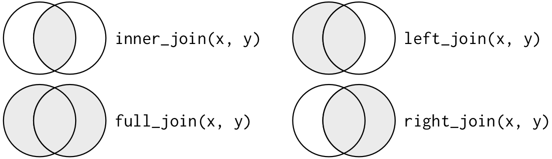
inner join: 只結合lhs rhs都有的
dplyr::inner_join()
left join: 只結合lhs有的
dplyr::left_join()
right join: 只結合rhs有的
dplyr::right_join()
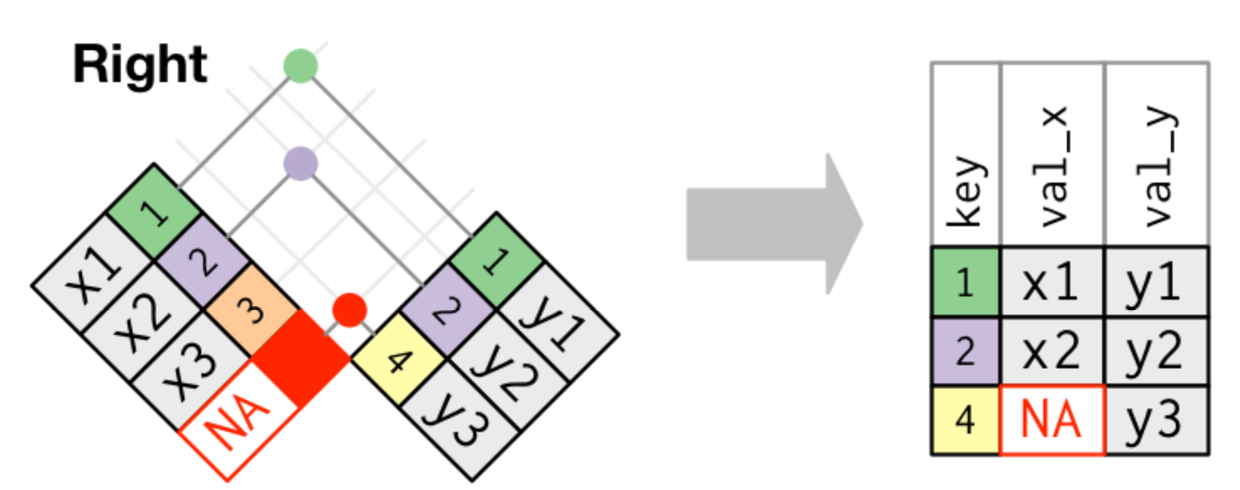
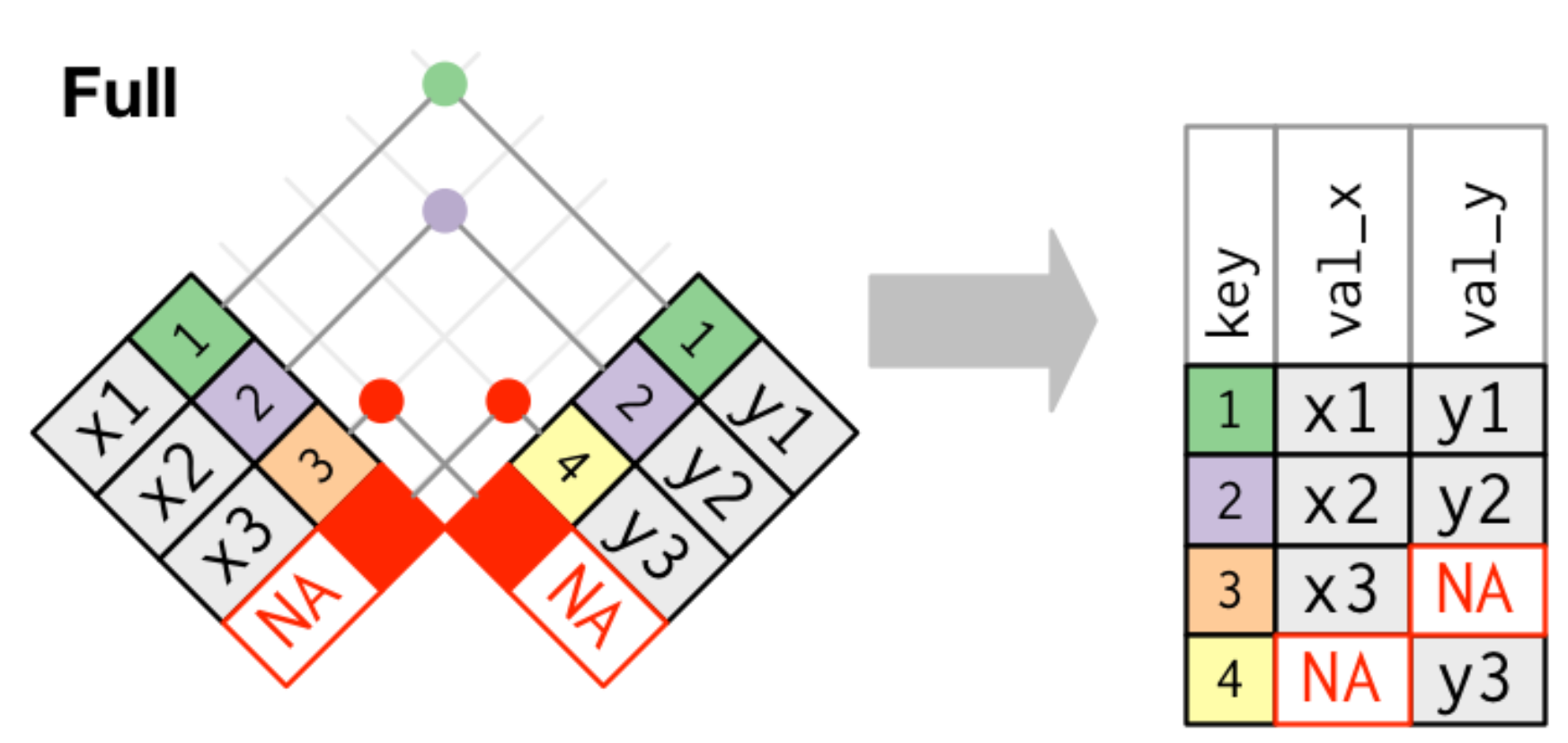
full join: 結合rhs&lhs有出現的
dplyr::full_join()
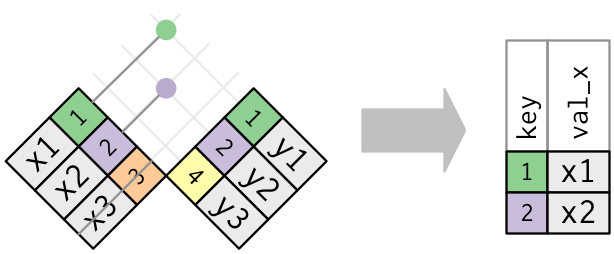
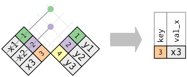
Duplicated keys
x <- tribble(
~key, ~val_x,
1, "x1",
2, "x2",
2, "x3",
1, "x4"
)
y <- tribble(
~key, ~val_y,
1, "y1",
2, "y2"
)
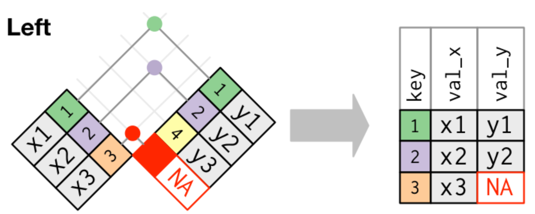
left_join(x, y, by = "key")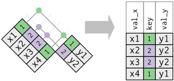
1. One table has duplicate keys.
2. Both tables have duplicate keys.
x <- tribble(
  ~key, ~val_x,
     1, "x1",
     2, "x2",
     2, "x3",
     3, "x4"
)
y <- tribble(
  ~key, ~val_y,
     1, "y1",
     2, "y2",
     2, "y3",
     3, "y4"
)
left_join(x, y, by = "key")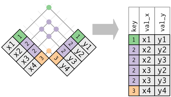
filtering joins
過濾結合: 匹配結合兩個資料表的觀察
semi join: 保留lhs在rhs匹配的所有觀察
dplyr::semi_join()
anti join: 捨棄lhs在rhs匹配的所有觀察
dplyr::anti_join()
Set Operations
Usage :
intersect(x, y, ...)
union(x, y, ...)
union_all(x, y, ...)
setdiff(x, y, ...)
setequal(x, y, ...)
df1 <- tribble(
  ~x, ~y,
   1,  1,
   2,  1
)
df2 <- tribble(
  ~x, ~y,
   1,  1,
   1,  2
)

intersect(df1, df2)
union(df1, df2)
setdiff(df1, df2)
setdiff(df2, df1)
intersect(df1, df2)
#> # A tibble: 1 x 2
#> x y
#> <dbl> <dbl>
#> 1 1 1
# Note that we get 3 rows, not 4
union(df1, df2)
#> # A tibble: 3 x 2
#> x y
#> <dbl> <dbl>
#> 1 1 2
#> 2 2 1
#> 3 1 1
setdiff(df1, df2)
#> # A tibble: 1 x 2
#> x y
#> <dbl> <dbl>
#> 1 2 1
setdiff(df2, df1)
#> # A tibble: 1 x 2
#> x y
#> <dbl> <dbl>
#> 1 1 2集合運算
本周作業~ Homework
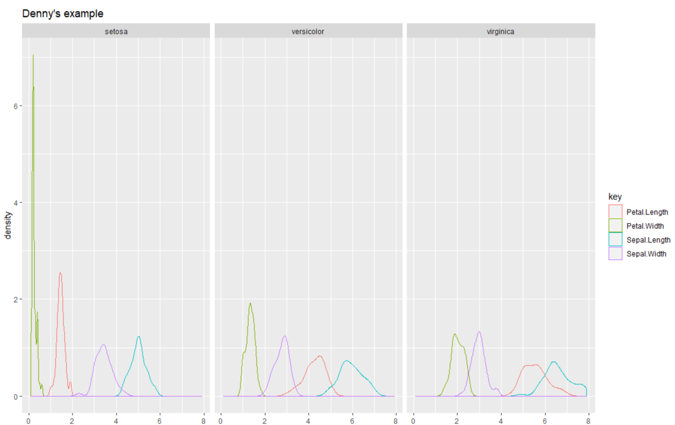
請"一次"將iris資料集,以面向(facet)將品種分別作圖,並將其餘數值型變數以密度圖表示,並且以顏色區分四種數值型變數,並且印出標題為各自的系級姓名。
Example
Tidyr Dplyr 12.02 教材
By Chen Ta Hung


