


Diego García Díaz
GIS & Remote Sensing. Python & Statistics. Surf & MTB :)
Curso: Google Earth Engine. Gabinete de Formación del CSIC.
Lugar: Estación Biológica de Doñana. Sevilla. 3-7/11/2025.
Profesor: Diego García Díaz.
Curso: Google Earth Engine. Gabinete de Formación del CSIC.
Lugar: Estación Biológica de Doñana. Sevilla. 3-7/11/2025.
Profesor: Diego García Díaz.
Curso: Google Earth Engine. Gabinete de Formación del CSIC.
Lugar: Estación Biológica de Doñana. Sevilla. 3-7/11/2025.
Profesor: Diego García Díaz.
Curso: Google Earth Engine. Gabinete de Formación del CSIC.
Lugar: Estación Biológica de Doñana. Sevilla. 3-7/11/2025.
Profesor: Diego García Díaz.
Curso: Google Earth Engine. Gabinete de Formación del CSIC.
Lugar: Estación Biológica de Doñana. Sevilla. 3-7/11/2025.
Profesor: Diego García Díaz.
Presentación del curso
Con suerte, aprenderemos un poco de todo
Curso: Google Earth Engine. Gabinete de Formación del CSIC.
Lugar: Estación Biológica de Doñana. Sevilla. 3-7/11/2025.
Profesor: Diego García Díaz.
Presentación del profe
Curso: Google Earth Engine. Gabinete de Formación del CSIC.
Lugar: Estación Biológica de Doñana. Sevilla. 3-7/11/2025.
Profesor: Diego García Díaz.
Presentación de los alumnos
Curso: Google Earth Engine. Gabinete de Formación del CSIC.
Lugar: Estación Biológica de Doñana. Sevilla. 3-7/11/2025.
Profesor: Diego García Díaz.
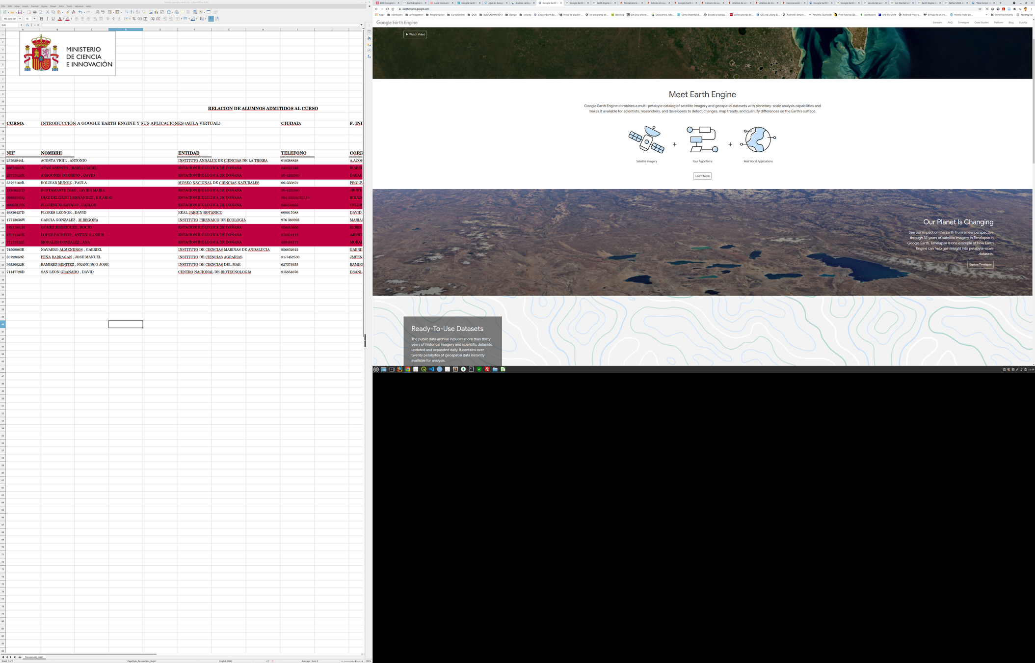
Introducción a Google Earth Engine
¡SERVIDOR DE IMÁGENES SATÉLITE!
¿Que es Google Earth Engine?
Respuesta Rápida:
Curso: Google Earth Engine. Gabinete de Formación del CSIC.
Lugar: Estación Biológica de Doñana. Sevilla. 3-7/11/2025.
Profesor: Diego García Díaz.
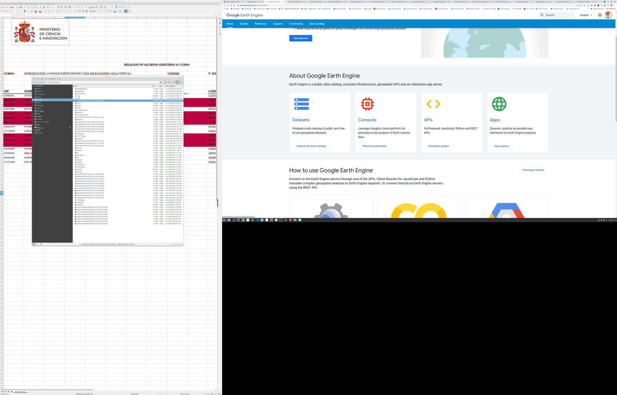
Introducción a Google Earth Engine
Earth Engine is a platform for scientific analysis and visualization of geospatial datasets,
for academic, non-profit, business and government users.
Earth Engine hosts satellite imagery and stores it in a public data archive that includes
historical earth images going back more than forty years. The images, ingested on a daily basis,
are then made available for global-scale data mining.
Earth Engine also provides APIs and other tools to enable the analysis of large datasets.
Curso: Google Earth Engine. Gabinete de Formación del CSIC.
Lugar: Estación Biológica de Doñana. Sevilla. 3-7/11/2025.
Profesor: Diego García Díaz.
Introducción a Google Earth Engine
TimeLapses
Datasets
API
Code Editor
Study Cases
Curso: Google Earth Engine. Gabinete de Formación del CSIC.
Lugar: Estación Biológica de Doñana. Sevilla. 3-7/11/2025.
Profesor: Diego García Díaz.
Introducción a Google Earth Engine
TimeLapses
Curso: Google Earth Engine. Gabinete de Formación del CSIC.
Lugar: Estación Biológica de Doñana. Sevilla. 3-7/11/2025.
Profesor: Diego García Díaz.
Introducción a Google Earth Engine
Datasets
Visualización y apertura en code-editor
Curso: Google Earth Engine. Gabinete de Formación del CSIC.
Lugar: Estación Biológica de Doñana. Sevilla. 3-7/11/2025.
Profesor: Diego García Díaz.
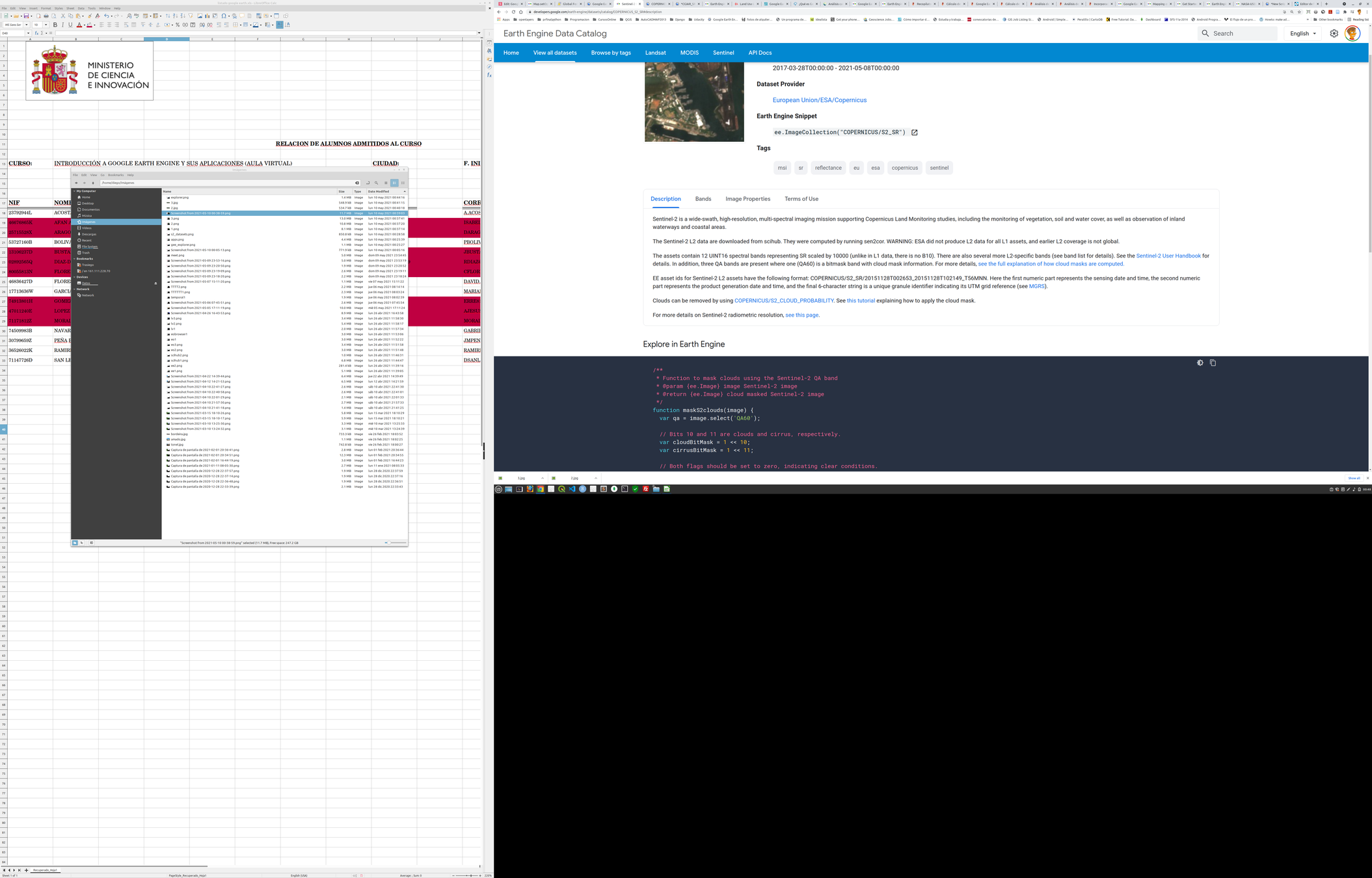
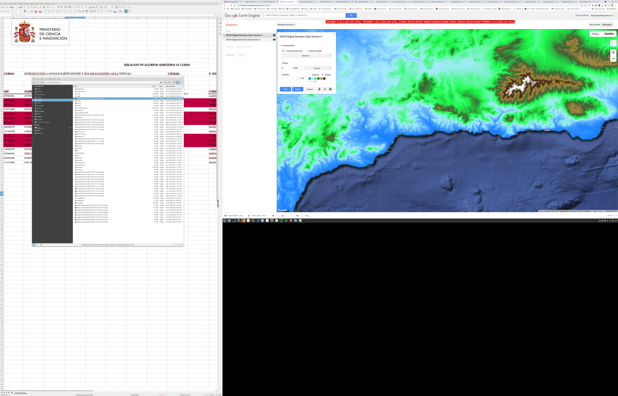
Introducción a Google Earth Engine
Datasets
Visualización y descarga en Explorer
Descarga
Curso: Google Earth Engine. Gabinete de Formación del CSIC.
Lugar: Estación Biológica de Doñana. Sevilla. 3-7/11/2025.
Profesor: Diego García Díaz.
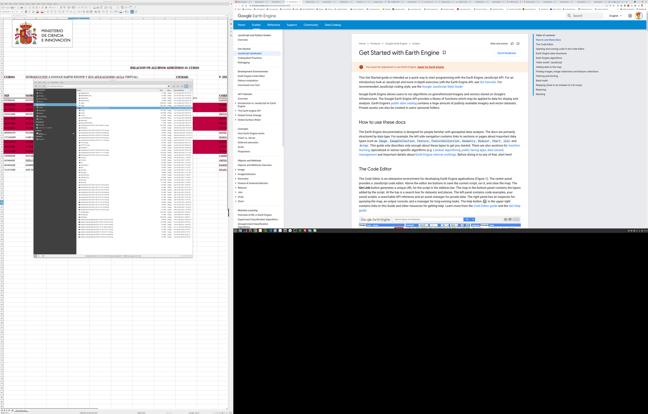
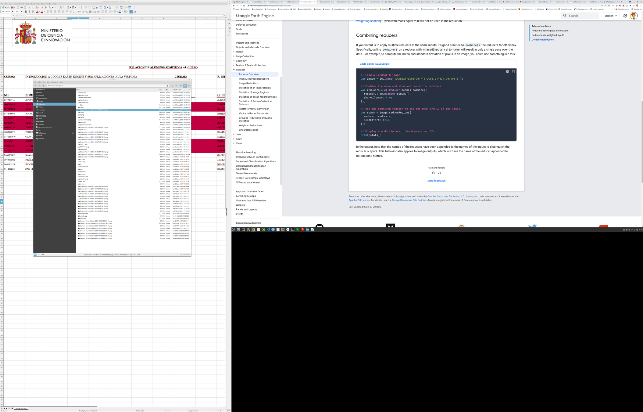
Introducción a Google Earth Engine
API
Se trata de la sección desde la que buscar toda la ayuda y las explicaciones sobre como programar para obtener el resultado que queremos
Curso: Google Earth Engine. Gabinete de Formación del CSIC.
Lugar: Estación Biológica de Doñana. Sevilla. 3-7/11/2025.
Profesor: Diego García Díaz.
https://www.google.com/intl/es_es/earth/outreach/learn/introduction-to-google-earth-engine/#earth-engine-explorer-0
Introducción a Google Earth Engine
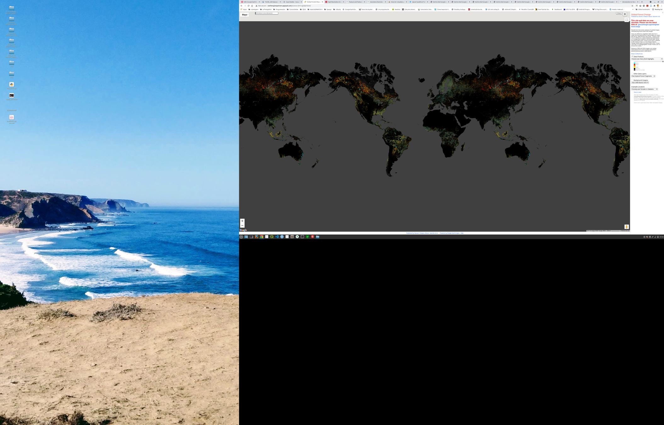
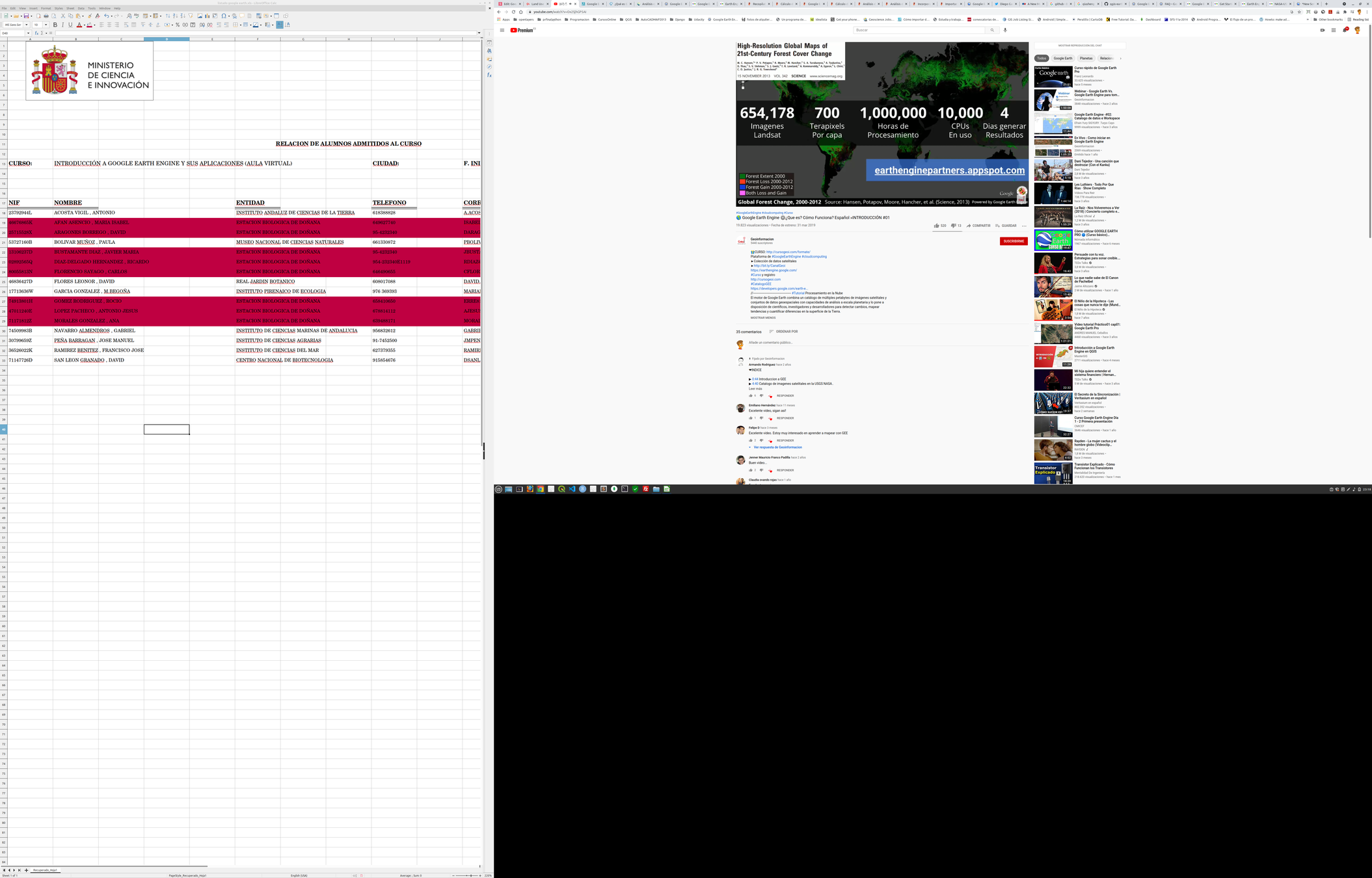
Study Cases
Global Forest Change
Curso: Google Earth Engine. Gabinete de Formación del CSIC.
Lugar: Estación Biológica de Doñana. Sevilla. 3-7/11/2025.
Profesor: Diego García Díaz.
Introducción a Google Earth Engine
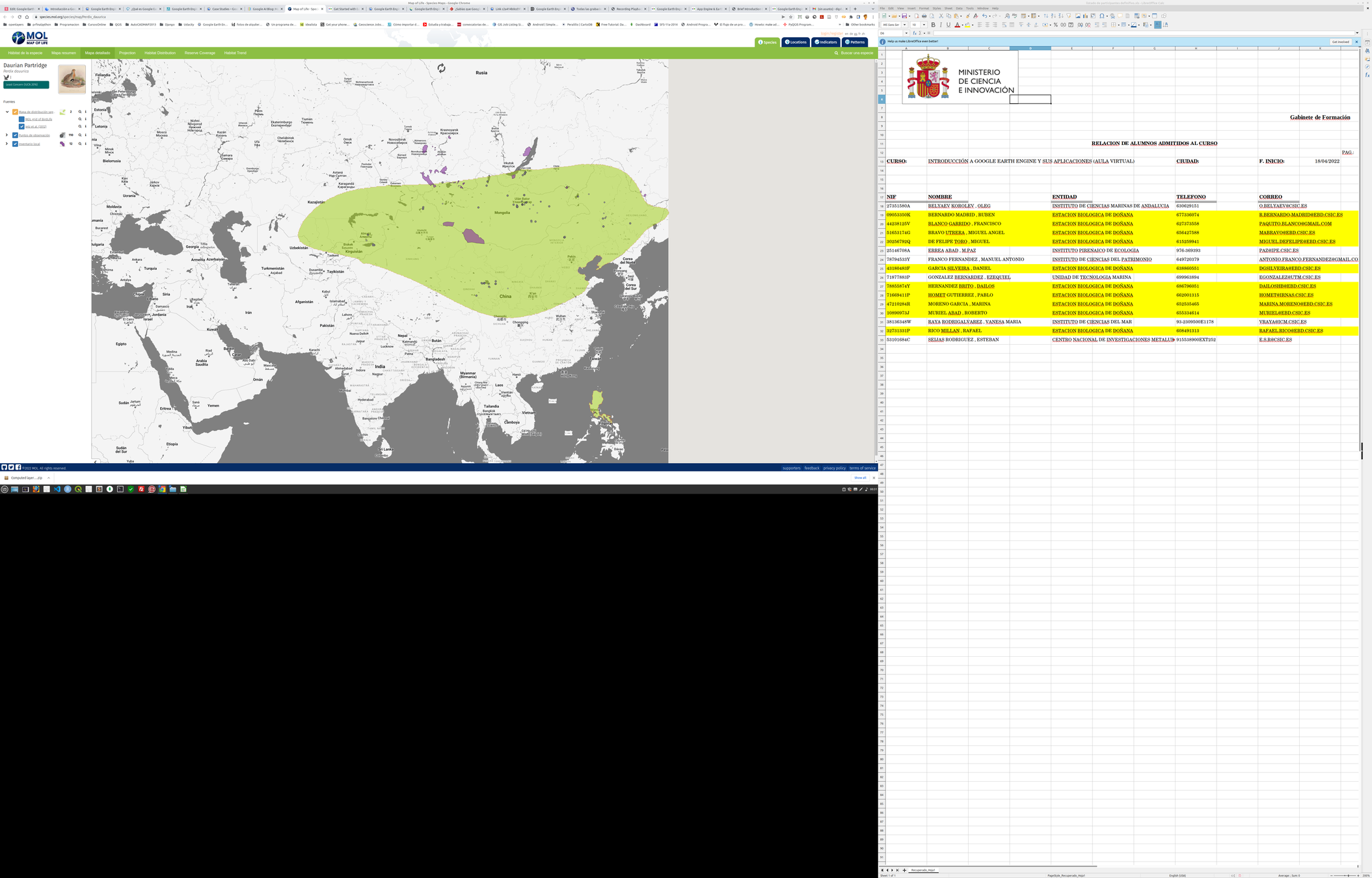
Study Cases
Map Of Life (MOL)
Curso: Google Earth Engine. Gabinete de Formación del CSIC.
Lugar: Estación Biológica de Doñana. Sevilla. 3-7/11/2025.
Profesor: Diego García Díaz.
Introducción a Google Earth Engine
Study Cases
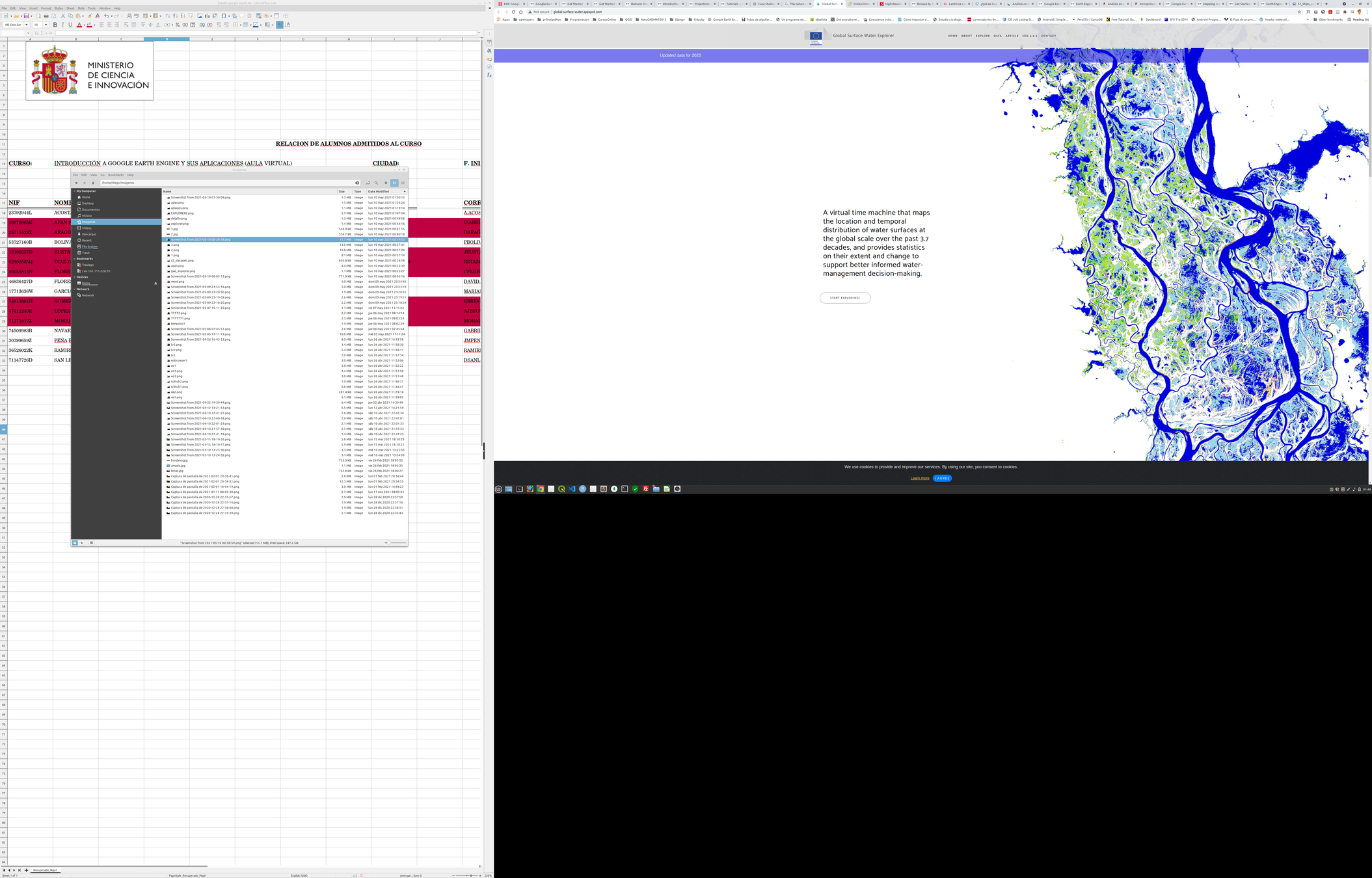
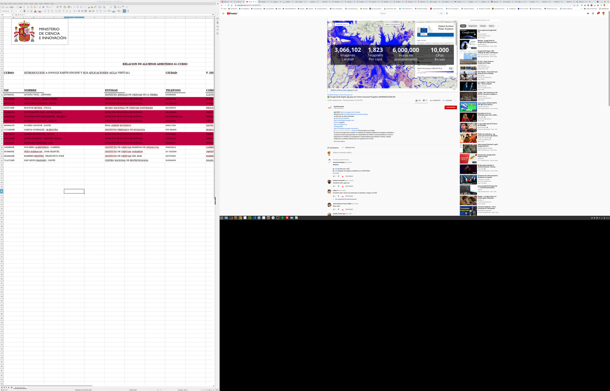
Global Water Occurence
Curso: Google Earth Engine. Gabinete de Formación del CSIC.
Lugar: Estación Biológica de Doñana. Sevilla. 3-7/11/2025.
Profesor: Diego García Díaz.
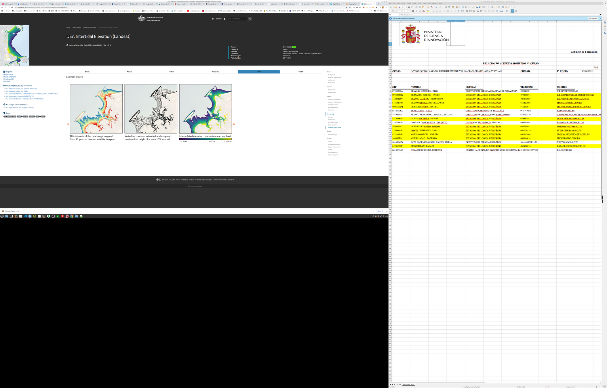
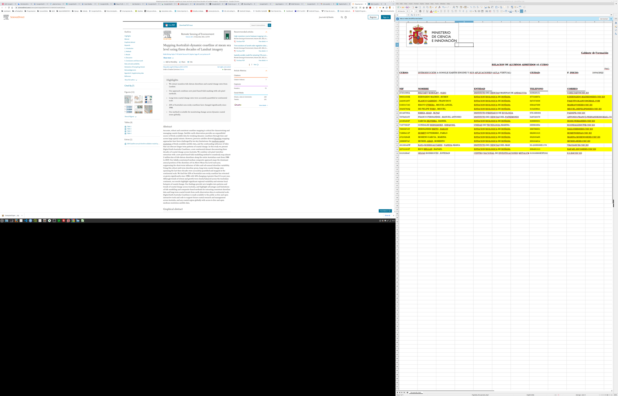
Introducción a Google Earth Engine
Study Cases
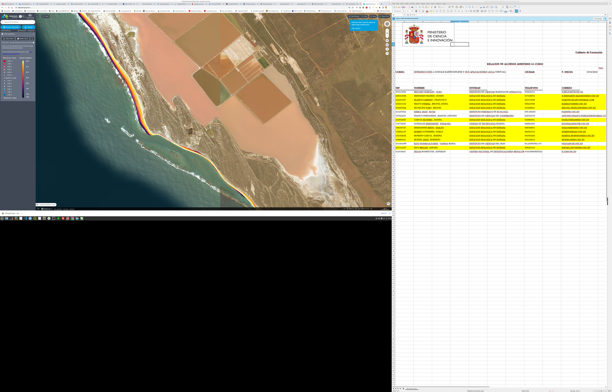
Digital Earth Australia (DEA) Shorelines & bathymetry
Curso: Google Earth Engine. Gabinete de Formación del CSIC.
Lugar: Estación Biológica de Doñana. Sevilla. 3-7/11/2025.
Profesor: Diego García Díaz.
Introducción a Google Earth Engine
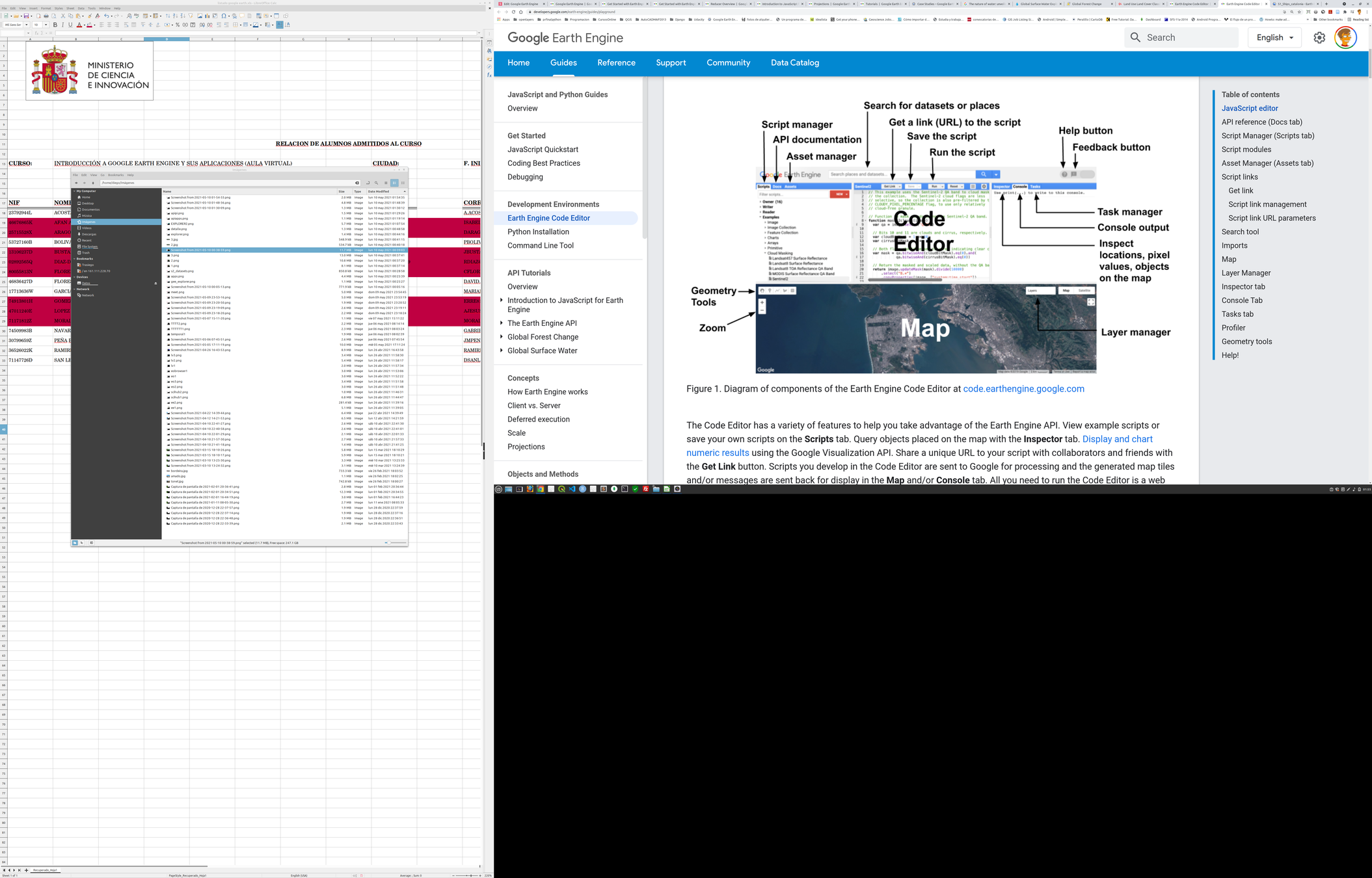
Code Editor
Curso: Google Earth Engine. Gabinete de Formación del CSIC.
Lugar: Estación Biológica de Doñana. Sevilla. 3-7/11/2025.
Profesor: Diego García Díaz.
Introducción a Google Earth Engine
Scripts
// Esto es un comentario de una línea
print('Hello world!');

/*
Esto es la apertura de un comentario multilinea

var saludo = 'Hello GEE world!';
print(saludo);

Esto es el cierre de un comentario multilinea

*/

var number = 99;
print('El número es ' + number);

var lista = [0,1,2,3,4,5];
print('La lista es: ', lista);

var lista2 = [6, 7, 8, 9, 10];
var lista3 = lista.concat(lista2);

lista.forEach(function(i) {
  print(i + 1)
});

print(lista3);

var Objeto = {
  name: 'Diego',
  notaMental: 'puh',
  edad: 43,
  hobbies: ['Mountain Bike', 'surf', 'llorar']
};

print('Dict:', Objeto);

// Function
var greet = function(name) {
    return 'Hello ' + name;
};
print(greet('World'));
Javascript Basico
Curso: Google Earth Engine. Gabinete de Formación del CSIC.
Lugar: Estación Biológica de Doñana. Sevilla. 3-7/11/2025.
Profesor: Diego García Díaz.
Introducción a Google Earth Engine
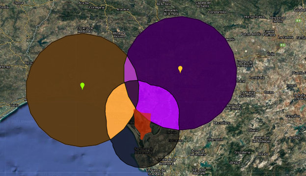
Scripts
var huelva_buffer = huelva.buffer(50000)
var sevilla_buffer = sevilla.buffer(50000)
var marisma_buffer = marisma.buffer(25000)

Map.addLayer(huelva_buffer, {color:'red'})
Map.addLayer(sevilla_buffer, {color:'blue'})


// Compute the intersection, display it in green.
var intersection = huelva_buffer.intersection(sevilla_buffer);
Map.addLayer(intersection, {color: '00FF00'}, 'intersection');

// Compute the union, display it in magenta.
var union = huelva_buffer.union(sevilla_buffer, ee.ErrorMargin(1));
Map.addLayer(union, {color: 'FF00FF'}, 'union');

// Compute the difference, display in yellow.
var diff1 = huelva_buffer.difference(sevilla_buffer, ee.ErrorMargin(1));
Map.addLayer(diff1, {color: 'FFFF00'}, 'diff1');

// Compute symmetric difference, display in black.
var symDiff = huelva_buffer.symmetricDifference(sevilla_buffer).symmetricDifference(marisma_buffer, ee.ErrorMargin(1));
Map.addLayer(symDiff, {color: '000000'}, 'symmetric difference');

print('El area de la marisma es', marisma.area())
print('El centroide se encuentra en', marisma.centroid())

Map.addLayer(marisma.centroid(), {}, 'Centroide')
Geometries
Curso: Google Earth Engine. Gabinete de Formación del CSIC.
Lugar: Estación Biológica de Doñana. Sevilla. 3-7/11/2025.
Profesor: Diego García Díaz.
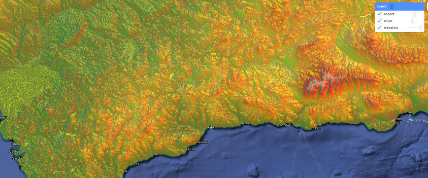
Introducción a Google Earth Engine
Scripts
//cargamos el datset como variable
var dataset = ee.Image('CGIAR/SRTM90_V4');

//seleccionamos la banda 'elevation'
var elevation = dataset.select('elevation');

//usamos las herramientas slope y aspect de la api disponibles en ee.Terrain (buscar en Docs)
var slope = ee.Terrain.slope(elevation);
var aspect = ee.Terrain.aspect(elevation);

//Añadimos el mapa y cargamos los rasters con su visualización. Cuidado de cargar la capa que es y cambiar los máximos y mínimos
Map.setCenter(-5.8598, 36.8841, 10);
Map.addLayer(elevation, {min: 0, max: 3000, palette: ['green', 'yellow', 'orange', 'brown', 'white']}, 'elevation');
Map.addLayer(slope, {min: 0, max: 45, palette: ['white', 'red']}, 'slope');
Map.addLayer(aspect, {min: 0, max: 360, palette: ['yellow', 'red', 'green', 'purple']}, 'aspect');
Terrain
Curso: Google Earth Engine. Gabinete de Formación del CSIC.
Lugar: Estación Biológica de Doñana. Sevilla. 3-7/11/2025.
Profesor: Diego García Díaz.
Introducción a Google Earth Engine
// IMPORTS
//Aquí tenemos que crear un polígono como geometría al que llamaremos roi para hacer el Zona Statistics (lineas 23-29)
//También tenemos que importar el shapefile de Andalucía, al que llamremos andalucia (linea 35)

//cargamos el datset como variable
var dataset = ee.Image('CGIAR/SRTM90_V4');

//seleccionamos la banda 'elevation'
var elevation = dataset.select('elevation');

//usamos las herramientas slope y aspect de la api disponibles en ee.Terrain (buscar en Docs)
var slope = ee.Terrain.slope(elevation);
var aspect = ee.Terrain.aspect(elevation);

//creamos una imagen compuesta con las 3 variables
var full = ee.Image.cat([elevation, slope, aspect]);

//Añadimos el mapa y cargamos los rasters con su visualización. Cuidado de cargar la capa que es y cambiar los máximos y mínimos
Map.setCenter(-5.8598, 36.8841, 10);
//Map.addLayer(elevation, {min: 0, max: 3000, palette: ['green', 'yellow', 'orange', 'brown', 'white']}, 'elevation');
//Map.addLayer(slope, {min: 0, max: 45, palette: ['white', 'red']}, 'slope');
//Map.addLayer(aspect, {min: 0, max: 360, palette: ['yellow', 'red', 'green', 'purple']}, 'aspect');
Map.addLayer(full, {min: 0, max:40, bands:['slope'], palette:['white', 'red']}, 'full_terrain');


//ESTADISTICAS ZONALES A UN ROI
var roiStats = full.reduceRegion({
  reducer: ee.Reducer.max(),
  geometry: roi,
  scale: 90,
  maxPixels: 1e9
});
print(roiStats)


//Estadisticas zonales a un municipio
var Almonte = andalucia.filter("nombre == 'Almonte'");
Map.addLayer(Almonte, {color: 'green'}, 'Almonte');

var AlmonteStats = full.reduceRegion({
  reducer: ee.Reducer.median(),
  geometry: Almonte,
  scale: 90,
  maxPixels: 1e9
});
print(AlmonteStats);


//Estadísticas zonales a la selección
var filtro = ee.Filter.inList('nombre', ['Almonte', 'Monachil', 'Cazorla']);
var munis = andalucia.filter(filtro);
Map.addLayer(munis, {color: 'purple'}, 'Municipios selected');

var selStats = full.select('elevation').reduceRegions({
    collection: munis.select(['nombre']),
    reducer: ee.Reducer.mean(),
    scale: 30})

print(selStats);

//con estas lineas vamos a visualizar todos los municipios sin relleno
var empty = ee.Image().byte();
// Paint all the polygon edges with the same number and width, display.
var outline = empty.paint({
  featureCollection: andalucia,
  //color: 5,
  width: 2
});
Map.addLayer(outline, {palette: 'black'}, 'edges');
Zonal Statistics (SRTM)
Curso: Google Earth Engine. Gabinete de Formación del CSIC.
Lugar: Estación Biológica de Doñana. Sevilla. 3-7/11/2025.
Profesor: Diego García Díaz.
Curso: Google Earth Engine. Gabinete de Formación del CSIC.
Lugar: Estación Biológica de Doñana. Sevilla. 4-8/11/2024.
Profesor: Diego García Díaz.
Curso: Google Earth Engine. Gabinete de Formación del CSIC.
Lugar: Estación Biológica de Doñana. Sevilla. 4-8/11/2024.
Profesor: Diego García Díaz.
// IMPORTS
//Aquí tenemos que crear un polígono como geometría al que llamaremos roi para hacer el Zona Statistics (lineas 23-29)
//También tenemos que importar el shapefile de Andalucía, al que llamremos andalucia (linea 35)

//cargamos el datset como variable
var dataset = ee.Image('CGIAR/SRTM90_V4');

//seleccionamos la banda 'elevation'
var elevation = dataset.select('elevation');

//usamos las herramientas slope y aspect de la api disponibles en ee.Terrain (buscar en Docs)
var slope = ee.Terrain.slope(elevation);
var aspect = ee.Terrain.aspect(elevation);

//creamos una imagen compuesta con las 3 variables
var full = ee.Image.cat([elevation, slope, aspect]);

//Añadimos el mapa y cargamos los rasters con su visualización. Cuidado de cargar la capa que es y cambiar los máximos y mínimos
Map.setCenter(-5.8598, 36.8841, 10);
//Map.addLayer(elevation, {min: 0, max: 3000, palette: ['green', 'yellow', 'orange', 'brown', 'white']}, 'elevation');
//Map.addLayer(slope, {min: 0, max: 45, palette: ['white', 'red']}, 'slope');
//Map.addLayer(aspect, {min: 0, max: 360, palette: ['yellow', 'red', 'green', 'purple']}, 'aspect');
Map.addLayer(full, {min: 0, max:40, bands:['slope'], palette:['white', 'red']}, 'full_terrain');


//ESTADISTICAS ZONALES A UN ROI
var roiStats = full.reduceRegion({
  reducer: ee.Reducer.max(),
  geometry: roi,
  scale: 90,
  maxPixels: 1e9
});
print(roiStats)


//Estadisticas zonales a un municipio
var Almonte = andalucia.filter("nombre == 'Almonte'");
Map.addLayer(Almonte, {color: 'green'}, 'Almonte');

var AlmonteStats = full.reduceRegion({
  reducer: ee.Reducer.median(),
  geometry: Almonte,
  scale: 90,
  maxPixels: 1e9
});
print(AlmonteStats);


//Estadísticas zonales a la selección
var filtro = ee.Filter.inList('nombre', ['Almonte', 'Monachil', 'Cazorla']);
var munis = andalucia.filter(filtro);
Map.addLayer(munis, {color: 'purple'}, 'Municipios selected');

var selStats = full.select('elevation').reduceRegions({
    collection: munis.select(['nombre']),
    reducer: ee.Reducer.mean(),
    scale: 30})

print(selStats);

//con estas lineas vamos a visualizar todos los municipios sin relleno
var empty = ee.Image().byte();
// Paint all the polygon edges with the same number and width, display.
var outline = empty.paint({
  featureCollection: andalucia,
  //color: 5,
  width: 2
});
Map.addLayer(outline, {palette: 'black'}, 'edges');
Zonal Statistics (SRTM)
// IMPORTS
//Aquí tenemos que crear un punto, lo usaremos para situarlo sobre la marisma (o la zona que queramos y que sea esa la que se cargue).
//Luego lo usaremos para hacer un buffer y un clip con el (lineas 8 y 54). Le dejaremos el nombre de geometry .

//Seleccionamos las imágenes Landsat en DNs (raw images) para aplicar el simpleComposite y reducir la colección  de Landsat con la imagen más limpia del año
var landsat = ee.ImageCollection("LANDSAT/LC08/C01/T1")
    .filterDate('2019-01-01', '2020-01-01')
    .filterBounds(geometry)

var composite = ee.Algorithms.Landsat.simpleComposite({
  collection: landsat,
  asFloat: true
})


// Compute NDVI 3 ways.
// Method 1)
var b5 = composite.select("B5")
var b4 = composite.select("B4")
var ndvi_1 = b5.subtract(b4).divide(b5.add(b4))

// Method 2)
var ndvi_2 = composite.normalizedDifference(["B5", "B4"])

// Method 3)
var ndvi_3 = composite.expression("(b5 - b4) / (b5 + b4)", {
    b5: composite.select("B5"),
    b4: composite.select("B4")
})

//Aqui estamos calculando la diferencia entre 2 métodos para calcualr el ndvi
var dif = ndvi_1.subtract(ndvi_2)

Map.addLayer(ndvi_1, {min:-0.2, max:0.8} , "NDVI")

Map.addLayer(dif, {min:-0.2, max:0.2} , "NDVI DIFF")

Map.centerObject(geometry, 10)

// Calculate Modified Normalized Difference Water Index (MNDWI)
var mndwi = composite.normalizedDifference(['B3', 'B6']).rename(['mndwi']);

// For more complex indices, you can use the expression() function
var savi = composite.expression(
    '1.5 * ((NIR - RED) / (NIR + RED + 0.5))', {
      'NIR': composite.select('B5'),
      'RED': composite.select('B4'),
}).rename('savi');

//var rgbVis = {min: 0.0, max: 350, bands: ['B5', 'B4', 'B3']};
var ndviVis = {min:0, max:1, palette: ['white', 'green']}
var ndwiVis = {min:0, max:0.5, palette: ['white', 'blue']}

Map.addLayer(mndwi.clip(geometry.buffer(25000), ndwiVis, 'mndwi')
Map.addLayer(savi, ndviVis, 'savi')
Image Calculations (Índices)
// IMPORTS
// Solo hay que crear un polígono con el área que queremos exportar. Le dejamos el nombre geometry (línea 37)

// Load an image collection, filtered so it's not too much data.
var collection = ee.ImageCollection('LANDSAT/LC08/C01/T1_SR')
  .filterDate('2017-05-01', '2017-06-30')
  //Aqui filtraríamos por path y row
  //.filter(ee.Filter.eq('WRS_PATH', 202))
  //.filter(ee.Filter.eq('WRS_ROW', 32));

// Compute the median in each band, each pixel.
// Band names are B1_median, B2_median, etc.
var ndvi = collection.map(function(image) {
  return image.select().addBands(image.normalizedDifference(['B5', 'B4']));
});

var median = ndvi.reduce(ee.Reducer.max());
var medianRGB = collection.reduce(ee.Reducer.median());

//paleta y parametros de visualización (diccionario) para el NDVI
var vis = {min: 0, max: 1, palette: [
  '0000FF', 'F8ECE0', 'FCD163', '66A000', '207401',
  '056201', '004C00', '023B01', '012E01', '011301'
]};

// The output is an Image.  Add it to the map.
var vis_param = {min: 500, max: 4500, bands: ['B5_median', 'B4_median', 'B3_median'], 'vis':vis, gamma: 1.6};
Map.centerObject(geometry, 8);
Map.addLayer(median, vis);
Map.addLayer(medianRGB,vis_param, 'RGB');


//Export to Image Drive
Export.image.toDrive({
  image: median,
  description: 'NDVI_L8_2017_median',
  scale: 30, //tamaño de pixel que queremos de salida.
  region: geometry,
  fileFormat: 'GeoTIFF',
  crs: 'EPSG:25830', //CRS de salida, nos permite reporyectar
  folder: 'Curso_GEE_CSIC' //si la carpeta no existiera la crearía. También podríamos exportar a Google Cloud o los Assets
  //maxPixels: 2000000000
});
Reducer and NDVI
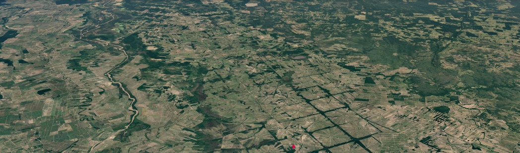
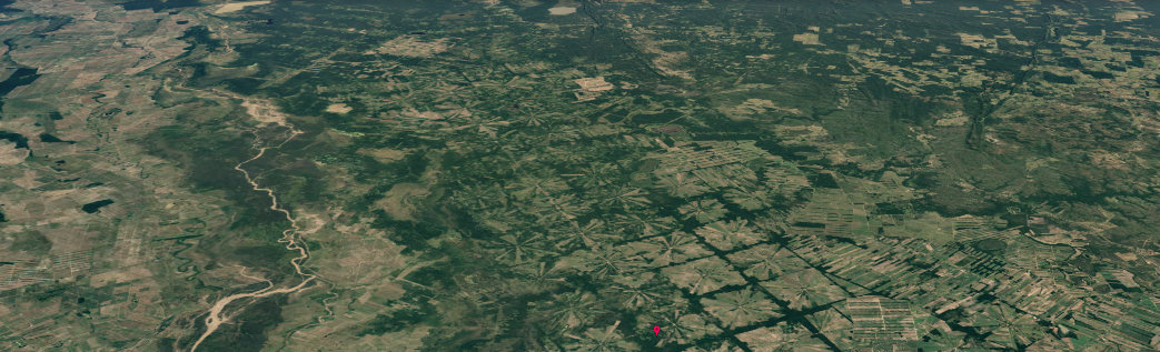
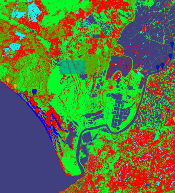
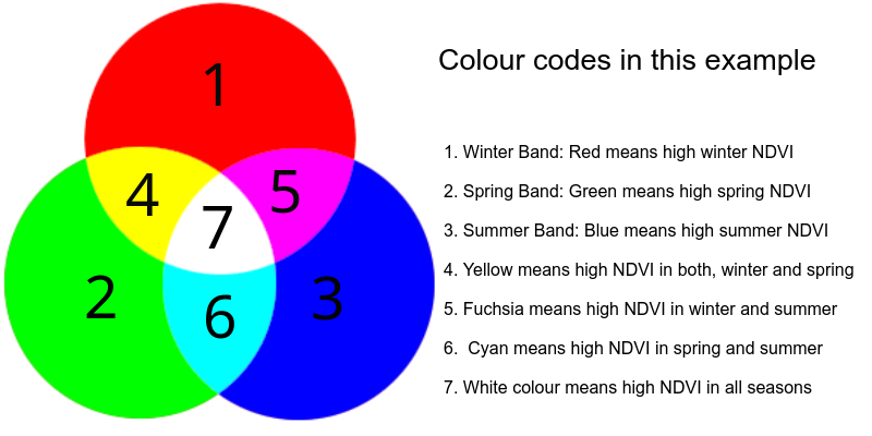
Vamos a realizar una composición de NDVI Multitemporal para ver la estacionalidad de los cultivos
Curso: Google Earth Engine. Gabinete de Formación del CSIC.
Lugar: Estación Biológica de Doñana. Sevilla. 4-8/11/2024.
Profesor: Diego García Díaz.
// IMPORTS
// Solo hay que crear un polígono con el área que queremos analizar. Le dejamos el nombre geometry.
// la idea es elegir una zona con muchos cultivos. En el desierto se ve muy bonito.

//Año 2016

var inv_16 = ee.ImageCollection('LANDSAT/LC08/C01/T1_32DAY_NDVI')
                  .filterDate('2016-01-01', '2016-03-31')
                  .select('NDVI').max();

var prim_16 = ee.ImageCollection('LANDSAT/LC08/C01/T1_32DAY_NDVI')
                  .filterDate('2016-04-01', '2016-06-30')
                  .select('NDVI').max();

var ver_16 = ee.ImageCollection('LANDSAT/LC08/C01/T1_32DAY_NDVI')
                  .filterDate('2016-07-01', '2016-09-30')
                  .select('NDVI').max();
//Año 2017

var inv_17 = ee.ImageCollection('LANDSAT/LC08/C01/T1_32DAY_NDVI')
                  .filterDate('2017-01-01', '2017-03-31')
                  .select('NDVI').max();

var prim_17 = ee.ImageCollection('LANDSAT/LC08/C01/T1_32DAY_NDVI')
                  .filterDate('2017-04-01', '2017-06-30')
                  .select('NDVI').max();

var ver_17 = ee.ImageCollection('LANDSAT/LC08/C01/T1_32DAY_NDVI')
                  .filterDate('2017-07-01', '2017-09-30')
                  .select('NDVI').max();
//Año 2018

var inv_18 = ee.ImageCollection('LANDSAT/LC08/C01/T1_32DAY_NDVI')
                  .filterDate('2018-01-01', '2018-03-31')
                  .select('NDVI').max();

var prim_18 = ee.ImageCollection('LANDSAT/LC08/C01/T1_32DAY_NDVI')
                  .filterDate('2018-04-01', '2018-06-30')
                  .select('NDVI').max();

var ver_18 = ee.ImageCollection('LANDSAT/LC08/C01/T1_32DAY_NDVI')
                  .filterDate('2018-07-01', '2018-09-30')
                  .select('NDVI').max();
//Año 2019

var inv_19 = ee.ImageCollection('LANDSAT/LC08/C01/T1_32DAY_NDVI')
                  .filterDate('2019-01-01', '2019-03-31')
                  .select('NDVI').max();

var prim_19 = ee.ImageCollection('LANDSAT/LC08/C01/T1_32DAY_NDVI')
                  .filterDate('2019-04-01', '2019-06-30')
                  .select('NDVI').max();

var ver_19 = ee.ImageCollection('LANDSAT/LC08/C01/T1_32DAY_NDVI')
                  .filterDate('2019-07-01', '2019-09-30')
                  .select('NDVI').max();


var year16 = ee.Image.cat(inv_16, prim_16, ver_16).clip(geometry); //si no hacemos clip tenemos el mundo entero
var year17 = ee.Image.cat(inv_17, prim_17, ver_17).clip(geometry);
var year18 = ee.Image.cat(inv_18, prim_18, ver_18).clip(geometry);
var year19 = ee.Image.cat(inv_19, prim_19, ver_19).clip(geometry);

//Aqui aplicamos un umbral a la de 2016 para que solo nos uestre los valores con el ndvi mayor de 0.25
var mean = year16.reduce(ee.Reducer.mean())
var mask = mean.gt(0.25);
var year_2016_masked = year16.mask(mask);
//var collection = ee.ImageCollection(year16).merge(year17).merge(year18).merge(year19);


Map.centerObject(geometry, 9);
Map.addLayer(year_2016_masked, {'min': 0.1, 'max': 0.7}, '2016');
Map.addLayer(geometry, {opacity: 0.7}, 'geometria');
Map.addLayer(year17, {'min': 0.1, 'max': 0.7}, '2017');
Map.addLayer(year18, {'min': 0.1, 'max': 0.7}, '2018');
//Map.addLayer(year19, {'min': 0.1, 'max': 0.7}, '2019');
NDVI Multitemporal
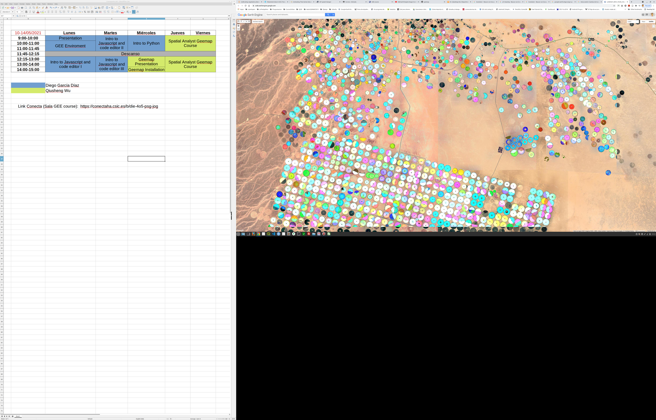
Vamos a combinar distintos datasets para obtener un producto mejorado. Usaremos datos de emisiones de luz y datos de población
Curso: Google Earth Engine. Gabinete de Formación del CSIC.
Lugar: Estación Biológica de Doñana. Sevilla. 4-8/11/2024.
Profesor: Diego García Díaz.
//Aqui no hay imports :)

//datset de población
var dataset = ee.Image('JRC/GHSL/P2016/BUILT_LDSMT_GLOBE_V1');
var builtUpMultitemporal = dataset.select('built')//.clip(country);

//datset de luces
var lights = ee.ImageCollection('NOAA/VIIRS/DNB/MONTHLY_V1/VCMSLCFG').select("avg_rad")
  .filter(ee.Filter.date('2014-01-01', '2014-12-31'));

//reducción de la serie anual con la suma y la mediana
var sum_Lights = lights.reduce(ee.Reducer.sum())//.clip(country);
var median_Lights = lights.reduce(ee.Reducer.median())//.clip(country);

//creamos y aplicamos el umbral como mascara para mejorar las zonas urbanas
var thold = median_Lights.gt(2);

var nthold = thold.mask(builtUpMultitemporal.gt(2));

var visParams = {
  min: 3.0,
  max: 6.0,
  palette: ['000000', 'D50606', 'F73131', 'F57474', 'F7B5B3'],
};


Map.setCenter(8.9957, 45.5718, 12);
Map.addLayer(builtUpMultitemporal, visParams, 'Built-Up Multitemporal');
Map.setCenter(20.1056, 20, 3);
Combinando Datsets (Población y Luces)
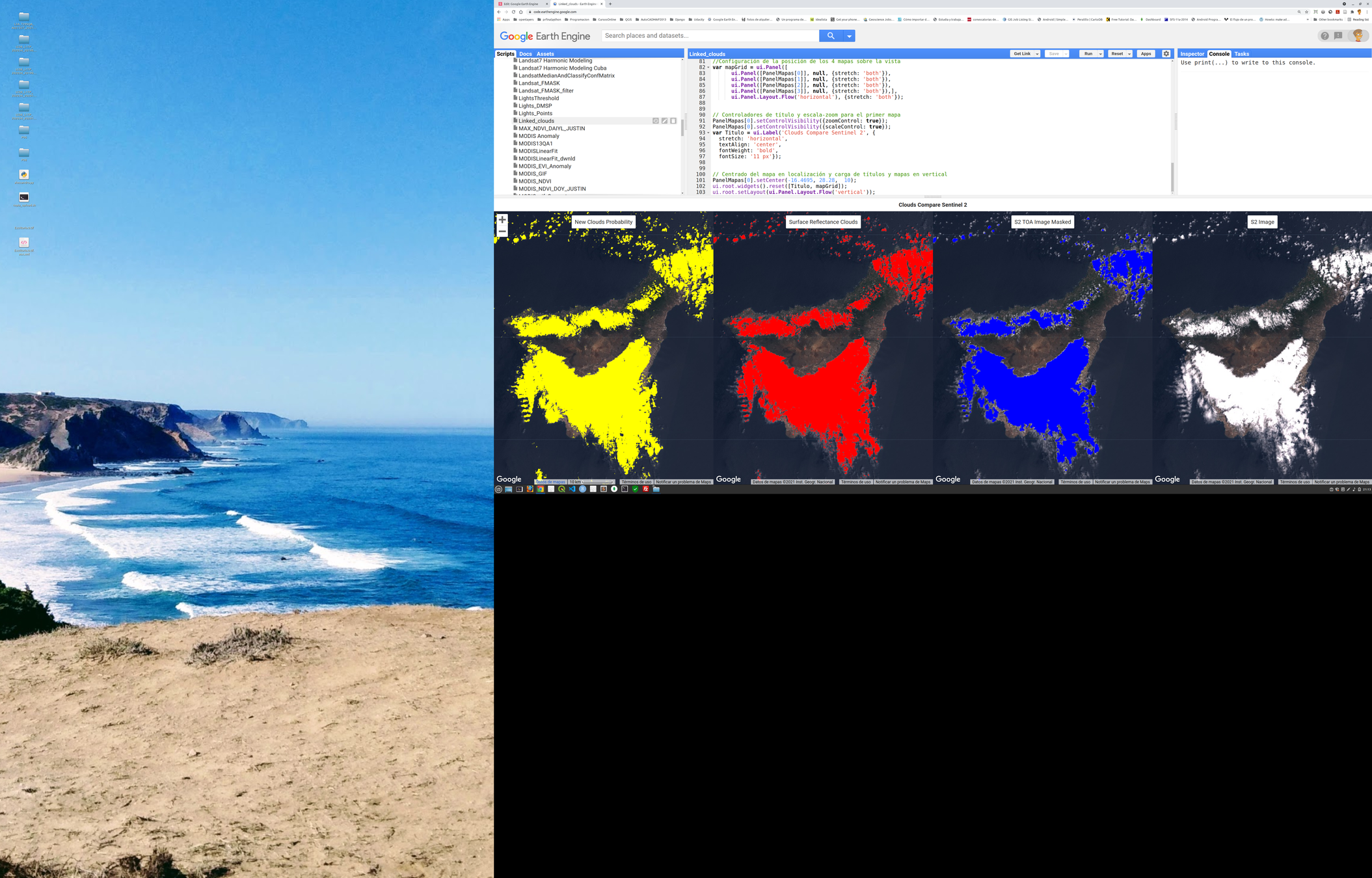
Vamos a combinar datos Sentinel 1 a lo largo de un periodo de tiempo largo para ver las rutas marítimas más utilizadas
Curso: Google Earth Engine. Gabinete de Formación del CSIC.
Lugar: Estación Biológica de Doñana. Sevilla. 4-8/11/2024.
Profesor: Diego García Díaz.
//Aqui tan solo creamos una geometría con la zona a la que queremos que nos haga zoom el mapa
//Le dejamos el nombre geometry (linea 81)

//var l8 = ee.ImageCollection("LANDSAT/LC08/C01/T1_SR");

// Function to cloud mask from the pixel_qa band of Landsat 8 SR data.
function maskL8sr(image) {
  // Bits 3 and 5 are cloud shadow and cloud, respectively.
  var cloudShadowBitMask = 1 << 3;
  var cloudsBitMask = 1 << 5;

  // Get the pixel QA band.
  var qa = image.select('pixel_qa');

  // Both flags should be set to zero, indicating clear conditions.
  var mask = qa.bitwiseAnd(cloudShadowBitMask).eq(0)
      .and(qa.bitwiseAnd(cloudsBitMask).eq(0));

  // Return the masked image, scaled to reflectance, without the QA bands.
  return image.updateMask(mask).divide(10000)
      .select("B[0-9]*")
      .copyProperties(image, ["system:time_start"]);
}

// Map the function over one year of data.
var collection = ee.ImageCollection('LANDSAT/LC08/C01/T1_SR')
    .filterDate('2020-01-01', '2020-12-31')
    .map(maskL8sr)

var composite = collection.median();

// Display the results.


// Get the median over time, in each band, in each pixel.
//var median = l8.filterDate('2020-01-01', '2020-12-31').median();
// Make a handy variable of visualization parameters.
var visParams = {bands: ['B6', 'B5', 'B4'], min: 100, max: 3500};

// Load or import the Hansen et al. forest change dataset.
var hansenImage = ee.Image('UMD/hansen/global_forest_change_2015');

// Select the land/water mask.
var datamask = hansenImage.select('datamask');

// Create a binary mask.
var mask = datamask.eq(1);
//var mask = datamask.eq(1);

// Update the composite mask with the water mask.
var maskedComposite = composite.updateMask(mask);
//Map.addLayer(maskedComposite, visParams, 'masked');


// Make a water image out of the mask.
var water = mask.not();
var land = mask.eq(1);

// Mask water with itself to mask all the zeros (non-water).
water = water.mask(water);
land = land.mask(land);

// Load the Sentinel-1 ImageCollection.
var sentinel1 = ee.ImageCollection('COPERNICUS/S1_GRD');

// Filter by metadata properties.
var vh_2020 = sentinel1
  // Filter to get images with VH polarization.
  .filter(ee.Filter.listContains('transmitterReceiverPolarisation', 'VH'))
  // Filter to get images collected in interferometric wide swath mode.
  .filter(ee.Filter.eq('instrumentMode', 'IW'))
  .filterDate("2020-01-01","2020-12-31");

// Filter to get images from different look angles.
var vhAscending = vh_2020.filter(ee.Filter.eq('orbitProperties_pass', 'ASCENDING'));
var vhDescending = vh_2020.filter(ee.Filter.eq('orbitProperties_pass', 'DESCENDING'));

var radar_2020 = vhAscending.select('VH').merge(vhDescending.select('VH')).max().mask(water);


// Map composite over the Channel
Map.centerObject(geometry, 12);
Map.addLayer(radar_2020, {min: -15, max: 0}, 'Radar Merge 2020');


composite = composite.mask(land);
Map.addLayer(composite, {bands: ['B5', 'B4', 'B3'], min: 0, max: 0.3}, 'Landsat composite');
SAR. Sentinel 1 Ships
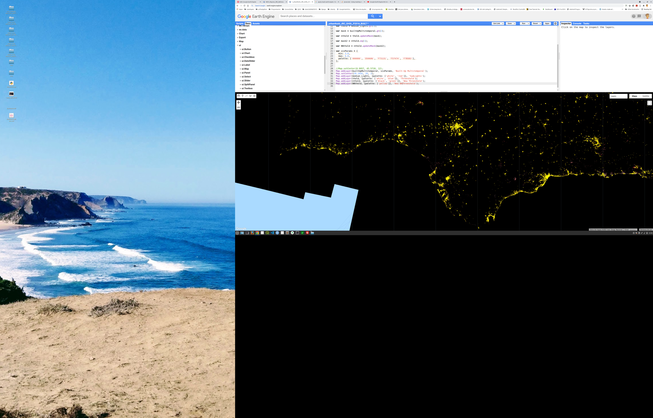
Vamos a crear una herramienta para comparar distintas máscaras de nubes disponibles para Sentinel 2
Curso: Google Earth Engine. Gabinete de Formación del CSIC.
Lugar: Estación Biológica de Doñana. Sevilla. 4-8/11/2024.
Profesor: Diego García Díaz.
//Aqui no hay imports

// Display a grid of linked maps, each with a different visualization.
var newclouds = ee.ImageCollection("COPERNICUS/S2_CLOUD_PROBABILITY")
  .filterDate('2018-05-01', '2018-05-05');

var s2sr = ee.ImageCollection("COPERNICUS/S2_SR")
  .select(['MSK_CLDPRB'])
  .filterDate('2018-05-01', '2018-05-05');

function greater(image) {
  var mask = image.gte(50)

  return image.updateMask(mask).eq(0)
}

var nclouds = newclouds.map(greater);
var srclouds = s2sr.map(greater);


function maskS2clouds(image) {
  var qa = image.select('QA60');

  // Bits 10 and 11 are clouds and cirrus, respectively.
  var cloudBitMask = 1 << 10;
  var cirrusBitMask = 1 << 11;

  // Both flags should be set to zero, indicating clear conditions.
  var mask = qa.bitwiseAnd(cloudBitMask).neq(0)
      //.and(qa.bitwiseAnd(cirrusBitMask).eq(0));

  return mask.updateMask(mask);
}

var s2 = ee.ImageCollection('COPERNICUS/S2')
                  .filterDate('2018-05-01', '2018-05-05')
                  //.map(maskS2clouds);

var q60_clouds = s2.map(maskS2clouds);

var rgbVis = {
  min: 0.0,
  max: 5000,
  bands: ['B4', 'B3', 'B2'],
};


//Creación y linkeo entre mapas
var PanelMapas = [];
//Object.keys(ComposicionesRGB).forEach(function(name) {
var Map1 = ui.Map();
Map1.add(ui.Label('New Clouds Probability'));
Map1.addLayer(s2, rgbVis, 'S2 Image');
Map1.addLayer(nclouds, {'min':0, 'max':100, 'palette':['yellow']}, 'New_Cloud Prob');
Map1.setControlVisibility(false);
PanelMapas.push(Map1);

var Map2 = ui.Map();
Map2.add(ui.Label('Surface Reflectance Clouds'));
Map2.addLayer(s2, rgbVis, 'S2 Image');
Map2.addLayer(srclouds, {'min':0, 'max':100, 'palette':['red']}, 'SR Clouds');
Map2.setControlVisibility(false);
PanelMapas.push(Map2);
User Interface Linked Maps
Curso: Google Earth Engine. Gabinete de Formación del CSIC.
Lugar: Estación Biológica de Doñana. Sevilla. 4-8/11/2024.
Profesor: Diego García Díaz.
Ejercicio:
Curso: Google Earth Engine. Gabinete de Formación del CSIC.
Lugar: Estación Biológica de Doñana. Sevilla. 4-8/11/2024.
Profesor: Diego García Díaz.
//IMPORTS
/* Aqui tendriamos que crear la feature collection con los puntos (geometrías en egenral) con los datos necesarios
para hacer la clasificación (deben tener un campo común que haga referencia a las clases). También podríamos subir
un shapefile a nuestro Assets y usarlo para hacer la clasificación
*/

// Partimos el año en estaciones o en nuestros periodos de interes

var sentinel2_winter = ee.ImageCollection("COPERNICUS/S2_SR")
    .filterDate('2018-01-01', '2018-03-31')
    .map(function(image) {
  return image.select().addBands(image.normalizedDifference(['B8', 'B4']).rename(['ndvi']))});
  //Con esta opción cogeríamos todas las bandas de Sentinel 2, junto con el NDVI
  //return image.select(['B2', 'B3', 'B4', 'B5', 'B6', 'B7', 'B8', 'B8A', 'B11', 'B12']).addBands(image.normalizedDifference(['B8', 'B4']).rename(['ndvi']))});

var sentinel2_spring = ee.ImageCollection("COPERNICUS/S2_SR")
    .filterDate('2018-04-01', '2018-06-30')
    .map(function(image) {
  return image.select().addBands(image.normalizedDifference(['B8', 'B4']).rename(['ndvi']))});
  //Con esta opción cogeríamos todas las bandas de Sentinel 2 junto con el NDVI
  //return image.select(['B2', 'B3', 'B4', 'B5', 'B6', 'B7', 'B8', 'B8A', 'B11', 'B12']).addBands(image.normalizedDifference(['B8', 'B4']).rename(['ndvi']))});
var sentinel2_summer = ee.ImageCollection("COPERNICUS/S2_SR")
    .filterDate('2018-07-01', '2018-09-30')
    .map(function(image) {
  return image.select().addBands(image.normalizedDifference(['B8', 'B4']).rename(['ndvi']))});
  //Con esta opción cogeríamos todas las bandas de Sentinel 2 junto con el NDVI
  //return image.select(['B2', 'B3', 'B4', 'B5', 'B6', 'B7', 'B8', 'B8A', 'B11', 'B12']).addBands(image.normalizedDifference(['B8', 'B4']).rename(['ndvi']))});

var sentinel2_autumn = ee.ImageCollection("COPERNICUS/S2_SR")
    .filterDate('2018-10-01', '2018-12-31')
    .map(function(image) {
  return image.select().addBands(image.normalizedDifference(['B8', 'B4']).rename(['ndvi']))});
  //Con esta opción cogeríamos todas las bandas de Sentinel 2 junto con el NDVI
  //return image.select(['B2', 'B3', 'B4', 'B5', 'B6', 'B7', 'B8', 'B8A', 'B11', 'B12']).addBands(image.normalizedDifference(['B8', 'B4']).rename(['ndvi']))});

//creamos la imagen compuesta con las 4 bandas
var ndvi_2018 = ee.Image.cat(sentinel2_winter.median(), sentinel2_spring.median(), sentinel2_summer.median(), sentinel2_autumn.median())

var vis = {min: 0, max: 0.8, palette: [
  'FFFFFF', 'CE7E45', 'FCD163', '66A000', '207401',
  '056201', '004C00', '023B01', '012E01', '011301'
]};

//añadimos la imagen con el NDVI multi temporal al mapa
Map.addLayer(ndvi_2018, {min:0, max:2000, bands:['B8', 'B4', 'B3']}, 'RGB');
Map.setCenter(-6.34497, 37.01918, 12);

// Merge the hand-drawn features into a single FeatureCollection.
var newfc = urbano.merge(pines).merge(water).merge(carliptos).merge(arenas).merge(greenhouse);

// Use these bands in the prediction.
var bands = ['ndvi', 'ndvi_1', 'ndvi_2', 'ndvi_3'];

//si usásemos todas las bandas quedaría así
/*var bands = ['B2', 'B3', 'B4', 'B5', 'B6', 'B7', 'B8', 'B8A', 'B11', 'B12', 'ndvi',
  'B2_1', 'B3_1', 'B4_1', 'B5_1', 'B6_1', 'B7_1', 'B8_1', 'B8A_1', 'B11_1', 'B12_1', 'ndvi_1',
  'B2_2', 'B3_2', 'B4_2', 'B5_2', 'B6_2', 'B7_2', 'B8_2', 'B8A_2', 'B11_2', 'B12_2''ndvi_2',
  'B2_3', 'B3_3', 'B4_3', 'B5_3', 'B6_3', 'B7_3', 'B8_3', 'B8A_3', 'B11_3', 'B12_3''ndvi_3'];
*/

// Creamos la capa de entrenamiento tomando los valores de éstas en las bandas de nuestro raster
var training = ndvi_2018.select(bands).sampleRegions({
  collection: newfc,
  properties: ['class'],
  scale: 10
});

// Seleccionamos un clasificador (ee.Classifier) y lo entrenamos con la capa creada en el paso anterior.
var classifier = ee.Classifier.smileCart().train({
  features: training,
  classProperty: 'class',
  inputProperties: bands
});

// Clasificamos la imagen.
var classified = ndvi_2018.select(bands).classify(classifier);

// Mostramos la clasificación en el mapa. Tened en cuenta el número de valores y que valor tiene cada clase para crear una paleta adecuada
Map.addLayer(classified, {min: 0, max: 6, palette: ['cyan', '00FF00', 'olive', 'blue', 'blue', 'red' ]}, 'classification');


// Validación
// Se crea una columna con valores random
var withRandom = training.randomColumn('random');

// En base a la columna random se parten los datos entre entrenamiento y test (para validar laclasificación).
var split = 0.7;  // El valor que usaremos para separar clasificación y test
var trainingPartition = withRandom.filter(ee.Filter.lt('random', split));
var testingPartition = withRandom.filter(ee.Filter.gte('random', split));

// Entrenamos el clasificador con nuestros datos para la clasificación (training partition)
var trainedClassifier = ee.Classifier.smileCart().train({
  features: trainingPartition,
  classProperty: 'class',
  inputProperties: bands
});

//clasificamos con el el clasificador entrenado con el 70% de los datos
var classified2 = ndvi_2018.classify(trainedClassifier);

//añadimos la clasifiación al mapa
Map.addLayer(classified2, {min: 0, max: 6, palette: ['cyan', '00FF00', 'olive', 'blue', 'blue', 'red']});

// Aquí es donde hacemos la clasificación con los datos de test, usando el clasificador entrenado con los datos de entrenamiento (linea 86)
//es aqui donde se genra el campo 'classification' que se usa en la matrix de confusión
var test = testingPartition.classify(trainedClassifier);

// Print the confusion matrix.
var confusionMatrix = test.errorMatrix('class', 'classification');
print('Confusion matrix:', confusionMatrix);
print('Overall Accuracy:', confusionMatrix.accuracy());
print('Producers Accuracy:', confusionMatrix.producersAccuracy());
print('Consumers Accuracy:', confusionMatrix.consumersAccuracy());Curso: Google Earth Engine. Gabinete de Formación del CSIC.
Lugar: Estación Biológica de Doñana. Sevilla. 4-8/11/2024.
Profesor: Diego García Díaz.
Curso: Google Earth Engine. Gabinete de Formación del CSIC.
Lugar: Estación Biológica de Doñana. Sevilla. 4-8/11/2024.
Profesor: Diego García Díaz.
Curso: Google Earth Engine. Gabinete de Formación del CSIC.
Lugar: Estación Biológica de Doñana. Sevilla. 4-8/11/2024.
Profesor: Diego García Díaz.
Geemap web: https://geemap.org/
Geemap Tutorials: https://geemap.org/tutorials/
Gee tutorials: https://tutorials.geemap.org/
Twitter: @giswqs
YouTube: https://blog.gishub.org/
Blog: https://blog.gishub.org/
Curso gratuito de Ujaval Gandhi (@spatialthoughts):
Cursos MOOC :
GEE tutorials :
Google Earth YouTube:
Twitter: @giswqs
Curso: Google Earth Engine. Gabinete de Formación del CSIC.
Lugar: Estación Biológica de Doñana. Sevilla. 4-8/11/2024.
Profesor: Diego García Díaz.
Documentación Oficial de Google Earth Engine:
Google Earth Engine Developers
La documentación oficial es uno de los mejores lugares para empezar. Incluye guías detalladas, ejemplos y una API Reference completa.
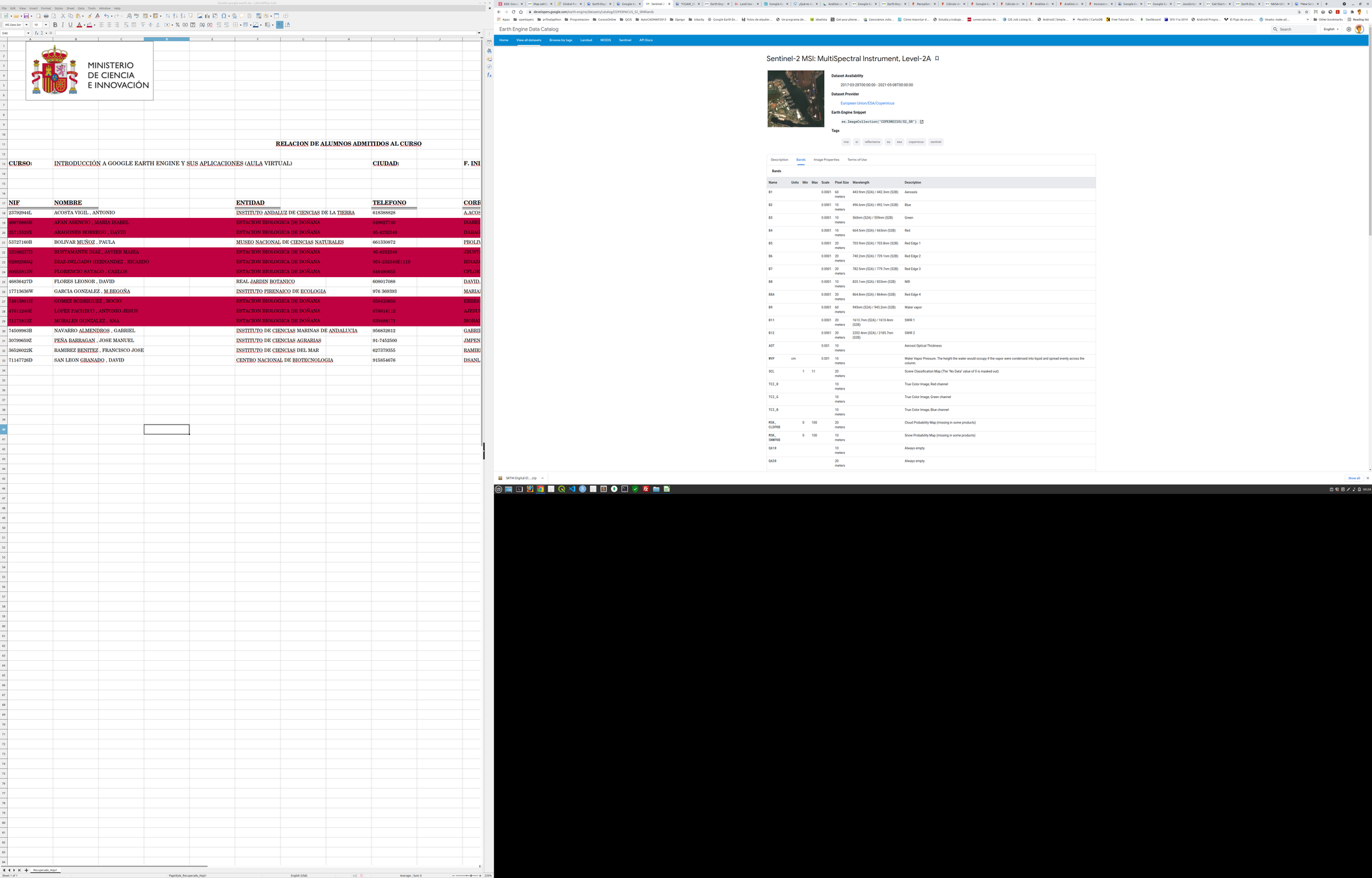
Earth Engine Data Catalog:
Google Earth Engine Data Catalog
Este catálogo te permite explorar los datos disponibles en GEE. Puedes buscar conjuntos de datos específicos de satélites, clima, hidrología, y más.
Cursos en Coursera y Udemy:
Earth Engine YouTube Channel:
Google Earth Engine YouTube
La serie de videos de Google Earth Engine en YouTube cubre desde aspectos básicos hasta técnicas avanzadas.
Foros y Comunidad de Usuarios:
google-earth-engine para encontrar soluciones a problemas específicos y tutoriales de otros desarrolladores.Tutoriales Avanzados en GitHub:
Awesome-GEE es una lista curada de bibliotecas y tutoriales que te ayudarán a realizar análisis complejos y explorar el potencial de GEE.
geemap Library:
geemap GitHub
Libraría de Python usada en el curso, para trabajar con GEE directamente desde el entorno Jupyter, añadiendo capacidades de mapa para la visualización y análisis de datos. Numerosos ejemplos prácticos con código incluido.
Curso: Google Earth Engine. Gabinete de Formación del CSIC.
Lugar: Estación Biológica de Doñana. Sevilla. 4-8/11/2024.
Profesor: Diego García Díaz.
https://freelearning.anaconda.cloud/get-started-with-anaconda
https://www.sciencedirect.com/science/article/pii/S0034425721004545?via%3Dihub
By Diego García Díaz


