Introduction to Generative Modeling

Francois Lanusse @EiffL

Do you know this person?

Probably not, this is a randomly generated person: thispersondoesntexist.com

What is generative modeling?

The goal of generative modeling is to learn the distribution from which the training set is drawn
Usually, this means building a parametric model that tries to be close to

X = \{ x_0, x_1, \ldots, x_N \}

p_\theta

True

samples

x \sim p

Model

p_\theta

Why it isn't that easy

The curse of dimensionality put all points far apart in high dimension
Classical methods for estimating probability densities, i.e. Kernel Density Estimation (KDE) start to fail in high dimension because of all the gaps

Distance between pairs of points drawn from a Gaussian distribution

So how do we get to this ?

Hint: Deep Learning is involved...

The Evolution of Deep Generative Models

Deep Belief Network
(Hinton et al. 2006)
Variational Auto-Encoder
(Kingma & Welling 2014)
Generative Adversarial Network
(Goodfellow et al. 2014)
Wasserstein GAN
(Arjovsky et al. 2017)

A Visual Turing Test

Fake images from a PixelCNN

Real SDSS images

How are these models usefull for physics?

They are data-driven models, can complement physical models

Lanusse et al. 2020

VAE model of galaxy morphology

They can learn from real data

They can learn from simulations

Mustafa et al. 2019

They can be orders of magnitude faster than a proper simulation and speed up significantly part of an analysis

Simulation of Dark Matter Maps

They can be used alongside physical model to solve diverse problems

Observations

Model convolved with PSF

Model

Residuals

Observed data

Imagined solutions

Boehm, Lanusse, Seljak 2019

DGM are a vast domain of research

Grathwohl et al. 2019

We will focus on a subset of Latent Variable Models today: GANs and VAEs

Latent Variable Models

We model using a mapping from a latent distribution to data space.
To draw a sample from , follow this recipe:
- Draw a latent variable z from a known/fixed distribution, e.g. a Gaussian, of low dimension:
- Transform this random variable to the data space using a deep neural network :
The goal of the game is to find the parameters so that ends up looking realistic.

p_\theta

z \sim \mathcal{N}(0, I)

g_\theta

p_\theta

g_\theta

x = g_\theta(z)

\theta

z \sim \mathcal{N}(0, I)

x = g_\theta(z)

Problem: In the data, I only have access to the output , but how can I train if I never see the input ????

Why do we expect this to work? We are saying that the data can actually be represented on the low dimensionality manifold in latent space.

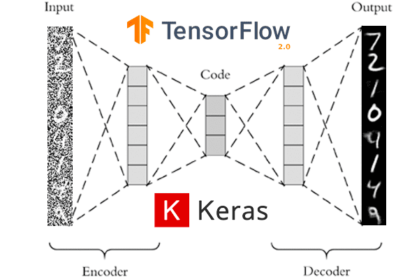
Part I: Auto-Encoders

The idea of auto-encoding:
Introduce a second network

The encoder tries to guess the latent variable that generates the image

Encoder

Decoder

\mathcal{L} = \parallel g_\theta( f_\phi(x) ) - x \parallel_2^2

The benefits of Auto-Encoding

Because the code is low-dimensional, it forces the model to compress the information as efficiently as possible in just a few numbers.

-> A great way to do dimensionality reduction

Auto-Encoded MNIST digits in 2d

Because they cannot preserve all of the information, they discard "noise", they can be used as denoisers
-> Denoising Auto-Encoders

Because they only know how to reconstruct a specific type of data, they will fail on an example from a different dataset
-> Anomaly detection

Examples in Physics:

Searching for New Physics with Deep Autoencoders, Farina et al. 2018
Variational Autoencoders for New Physics Mining
at the Large Hadron Collider, Cerri et al. 2019

Let's try it out!

Guided tutorial on Colab at this link.

Main Takeaway

Auto-Encoders can work very well to compress data
They can't be directly used as generative models because we don't know a priori how the latent space gets distributed

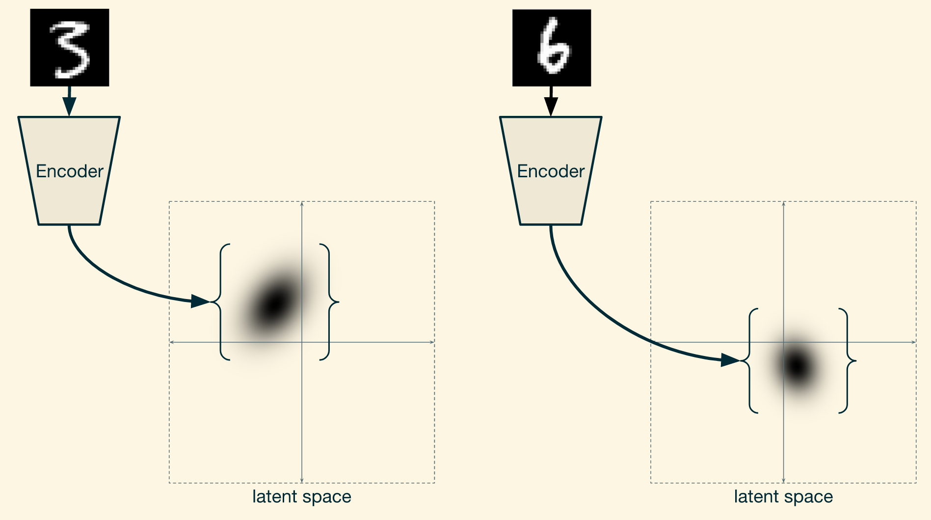
Part II: Variational Auto-Encoders

What is the difference to a normal Auto-Encoder?

An Auto-Encoder has only one constraint: Encode and then Decode has best you can:

-> We never ask it to make sure that the latent variables follow a particular distribution.
If the latent space has regularity.... it's only by chance

\mathcal{L} = \parallel g_\theta( f_\phi(x) ) - x \parallel_2^2

z= f_\phi(x)

A Variational Auto-Encoder tries to make sure that the latent variable follows a desired prior distribution:

because if we know that the latent space of the auto-encoder is Gaussian distributed, we can sample from it.
To achieve this, a VAE is trained using the Evidence Lower Bound (ELBO):

z \sim \mathcal{N}(0, I)

p_{\theta, \phi}(x) \geq \mathbb{E}_{z \sim q(.|x) }\left[ \log p_\theta(x | z) \right] - D_\mathrm{KL}\left(q_\phi(z | x) \parallel p(z)\right)

Reconstruction Error

Code Regularization

Unpacking the ELBO

p_{\theta, \phi}(x) \geq \mathbb{E}_{z \sim q_\phi(.|x) }\left[ \log p_\theta(x | z) \right] - D_\mathrm{KL}\left(q_\phi(z | x) \parallel p(z)\right)

The Likelihood term
-> Probability of image if is known.
- This needs to assume some knowledge of the statistics of the signal x

\log p_\theta(x | z)

p_\theta(x |z) = \mathrm{Bernoulli}( x | p=g_\theta(z) )

p_\theta(x |z) = \mathcal{N}( x | \mu=g_\theta(z); \Sigma=\sigma^2 I )

In this case, this is equivalent to the AE loss if

\sigma=1

\mathcal{L}_{AE} = \parallel g_\theta( z ) - x \parallel_2^2

Unpacking the ELBO

p_{\theta, \phi}(x) \geq \mathbb{E}_{z \sim q_\phi(.|x) }\left[ \log p_\theta(x | z) \right] - D_\mathrm{KL}\left(q_\phi(z | x) \parallel p(z)\right)

The Posterior
-> Tries to estimate the probability of if image is known
This is what the encoder models.

q_\phi(z | x)

The Kullback-Leibler Divergence

Image credit

A distance between distributions: the Kullback-Leibler Divergence

credit

Unpacking the ELBO

p_{\theta, \phi}(x) \geq \mathbb{E}_{z \sim q_\phi(.|x) }\left[ \log p_\theta(x | z) \right] - D_\mathrm{KL}\left(q_\phi(z | x) \parallel p(z)\right)

The ELBO is maximal when the input x is close to the output, and the code is close to a Gaussian

Reconstruction Error

Code Regularization

How do we build a network that outputs distributions?

q_\phi(z | x)

Tensorflow Probability

import tensorflow as tf
import tensorflow_probability as tfp
tfd = tfp.distributions

# Build model.
model = tf.keras.Sequential([
  tf.keras.layers.Dense(1+1),
  tfp.layers.IndependentNormal(1),
])

# Define the loss function:
negloglik = lambda x, q: - q.log_prob(x)

# Do inference.
model.compile(optimizer='adam', loss=negloglik)
model.fit(x, y, epochs=500)

# Make predictions.
yhat = model(x_tst)

Let's try it out!

Guided tutorial on Colab at this link.

Part III: Generative Adversarial Networks

What is a GAN?

It is again a Latent Variable Model

Contrary to a VAE, a GAN does not try to bound or estimate , instead the parameters are estimated by Adversarial Training.

p_\theta(x)

z \sim \mathcal{N}(0, I)

x = g_\theta(z)

x \sim p(x)

x \sim p_\theta(x)

The Discriminator is trained to classify between real and fake images
The Generator is trained to generate images that the discriminator will think are real

\arg\max_{\phi} \log d_\phi(x) + \log(1 - d_\phi(g_\theta(z)))

\arg\min_{\theta} \log(1 - d_\phi(g_\theta(z)))

Traditional GAN (Goodfellow 2014)

Spoiler Alert: GANs are difficult to train

In this competition between generator and discriminator, you have to make sure they are of similar strength.
Typically training is not convergent, the GAN doesn't settle in a solution but is constently shifting. You may get better results in the middle of training than at the end!
Beware of mode collapse!

BigGAN

VQ-VAE

Razavi et al. 2019

Vanishing gradients far from data distribution

Arjovsky et al. 2017

WGAN-GP: Your Go-To GAN

The discriminator/critic is computing a distance between two distributions (of real and fake images), a Wasserstein distance (hence the W).
-> This requires certain constraints on the critic (that's where the GP comes in).
The generator is trying to minimize that distance

Gulrajani et al. 2017

Training of the WGAN is still efficient even when the two distrtibutions are far apart.

What is this GP-thing?

For the derivation of the WGAN to work, it requires a Lipschitz bound on the critic.
The Gradient Penalty is a way to impose that condition on the critic

How far will this take us?

128x128 images, state of the art in 2017

WGAN-GP

StyleGAN2

1024x1024, state of the art circa end of 2019

This is extremely compute expensive and extremely technical

Let's try it out!

Guided tutorial on Colab at this link.

Introduction to Generative Modeling

What is generative modeling?

Why it isn't that easy

So how do we get to this ?

The Evolution of Deep Generative Models

A Visual Turing Test

How are these models usefull for physics?

DGM are a vast domain of research

Latent Variable Models

Part I: Auto-Encoders

The idea of auto-encoding: Introduce a second network

The benefits of Auto-Encoding

Let's try it out!

Main Takeaway

Part II: Variational Auto-Encoders

What is the difference to a normal Auto-Encoder?

Unpacking the ELBO

Unpacking the ELBO

Unpacking the ELBO

How do we build a network that outputs distributions?

Let's try it out!

Part III: Generative Adversarial Networks

What is a GAN?

Spoiler Alert: GANs are difficult to train

WGAN-GP: Your Go-To GAN

What is this GP-thing?

How far will this take us?

Let's try it out!

Introduction to Generative Modeling

More from eiffl

The idea of auto-encoding:
Introduce a second network