Introduction to Deep Probabilistic Learning

ML Sesion @ Astro Hack Week 2019

Francois Lanusse @EiffL

Gabriella Contardo @contardog

+ p(x) =

Follow the slides live at

https://slides.com/eiffl/tf_proba/live

q_\varphi(\theta= \mathrm{cat} | x) = 0.9

credit: Venkatesh Tata

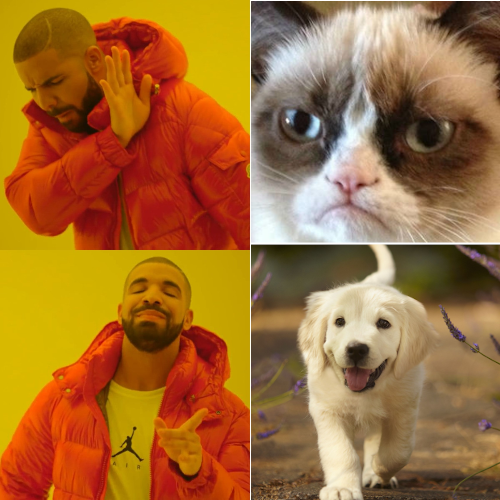
Let's start with binary classification

\theta

=> This means expressing the posterior as a Bernoulli distribution with parameter predicted by a neural network

How do we adjust this parametric distribution to match the true posterior ?

Step 1: We neeed some data

\mathcal{D} = \{ (x_i, \theta_i) \}_{i \in [0, N]}

cat or dog image

label 1 for cat, 0 for dog

(x, \theta) \sim p(x, \theta) = \tilde{p}(\theta) p(x | \theta)

Probability of including cats and dogs in my dataset

Google Image search results for cats and dogs

How do we adjust this parametric distribution to match the true posterior ?

A distance between distributions: the Kullback-Leibler Divergence

credit

D_{KL} (p || q) = \mathbb{E}_{x \sim p(x)} \left[ \log \frac{p(x)}{q(x)} \right]

Step 2: We need a tool to compare distributions

D_{KL} \left( p(x, \theta) || q_\varphi(\theta | x) \tilde{p}(x) \right) = - \mathbb{E}_{p(x,\theta)} \left[ \log \frac{ q_\varphi(\theta | x) \tilde{p}(x) }{ \tilde{p}(\theta) p(x | \theta) } \right]

= - \mathbb{E}_{p(x, \theta)} \left[ \log q_\varphi(\theta | x) \right] + cst

Minimizing this KL divergence is equivalent to minimizing the negative log likelihood of the model

D_{KL} \left( p(x, \theta) || q_\varphi(\theta | x) \tilde{p}(x) \right) = 0 \ <=> \ q_\varphi(\theta | x) \propto \frac{\tilde{p}(\theta)}{p(\theta)} p(\theta | x)

At minimum negative log likelihood, up to a prior term, the model recovers the Bayesian posterior

p(\theta | x) \propto p(x | \theta) p(\theta)

with

How do we adjust this parametric distribution to match the true posterior ?

In our case of binary classification:

\mathbb{E}_{p(x,\theta)}[ - \log q_\varphi(\theta | x)] =\\ \sum_{i=1}^{N} p(1|x_i) \log q_\varphi(1 | x_i) + (1-p(1|x_i)) \log_\varphi(1 | x_i)

We recover the binary cross entropy loss function !

The Probabilistic Deep Learning Recipe

Express the output of the model as a distribution
Optimize for the negative log likelihood
Maybe adjust by a ratio of proposal to prior if the training set is not distributed according to the prior
Profit!

q_\varphi(\theta | x)

\mathcal{L} = - \log q_\varphi(\theta | x)

q_\varphi(\theta | x) \propto \frac{\tilde{p}(\theta)}{p(\theta)} p(\theta | x)

How do we do this in practice?

Tensorflow Probability

import tensorflow as tf
import tensorflow_probability as tfp
tfd = tfp.distributions

# Build model.
model = tf.keras.Sequential([
  tf.keras.layers.Dense(1+1),
  tfp.layers.IndependentNormal(1),
])

# Define the loss function:
negloglik = lambda x, q: - q.log_prob(x)

# Do inference.
model.compile(optimizer='adam', loss=negloglik)
model.fit(x, y, epochs=500)

# Make predictions.
yhat = model(x_tst)

Let's try it out!

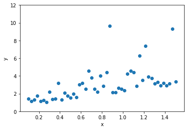
This is our data

Build a regression model for y gvien x

import tensorflow.keras as keras
import tensorflow_probability as tfp

# Number of components in the Gaussian Mixture
num_components = 16

# Shape of the distribution
event_shape = [1]

# Utility function to compute how many parameters this distribution requires

params_size = tfp.layers.MixtureNormal.params_size(num_components, event_shape)

gmm_model = keras.Sequential([
    keras.layers.Dense(units=128, activation='relu', input_shape=(1,)),
    keras.layers.Dense(units=128, activation='tanh'),
    keras.layers.Dense(params_size),
    tfp.layers.MixtureNormal(num_components, event_shape)
])

negloglik = lambda y, q: -q.log_prob(y)

gmm_model.compile(loss=negloglik, optimizer='adam')

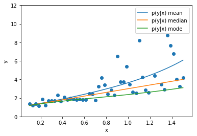
gmm_model.fit(x_train.reshape((-1,1)), y_train.reshape((-1,1)), 
              batch_size=256, epochs=20)

Link to Notebook