Hybrid Forward Models and Efficient Inference
Putting the Cosmic Large-scale Structure on the Map: Theory Meets Numerics
Sept. 2025
François Lanusse
Université Paris-Saclay, Université Paris Cité, CEA, CNRS, AIM

It's all about Simulation-Based Inference
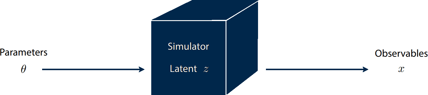
Implicit Simulation-Based Inference
Explicit Simulation-Based Inference
(x, \theta) \sim p(x, \theta)
p(\theta, z) \propto p(x | z, \theta) p(z, \theta) p(\theta)
a.k.a:
- Implicit Likelihood Inference (ILI)
- Simulation Based Inference (SBI)
- Likelihood-free Inference (LFI)
- Approximate Bayesian Computation (ABC)
a.k.a:
- Bayesian Hierarchical Modeling (BHM)
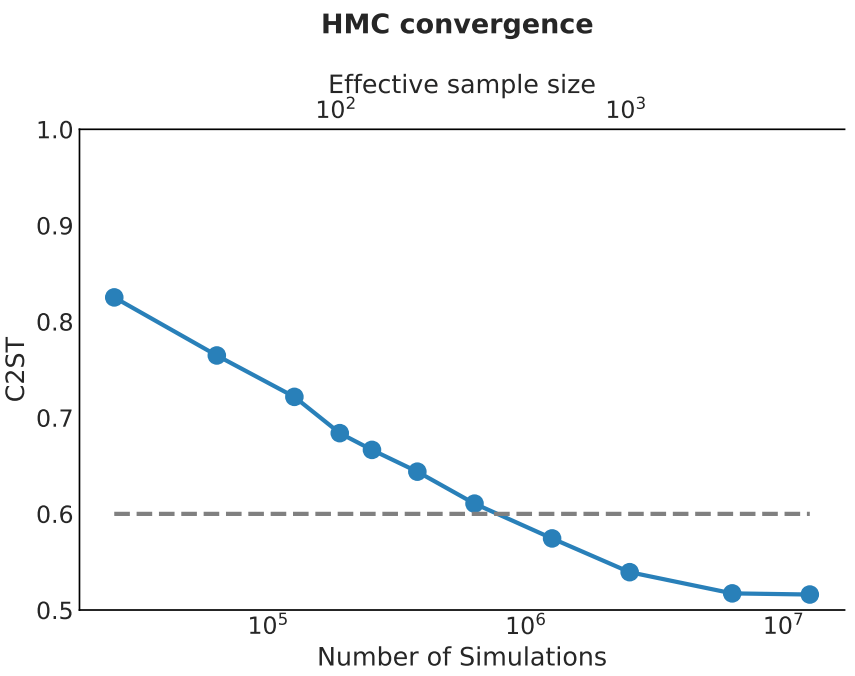
Which One is Better?
A few things to note:
- Both methods will give you exactly the same result given the same simulation model.
- Implicit inference is vastly more simulation-efficient than naive HMC sampling.
Dr. Justine Zeghal
(now at U. of Montreal)
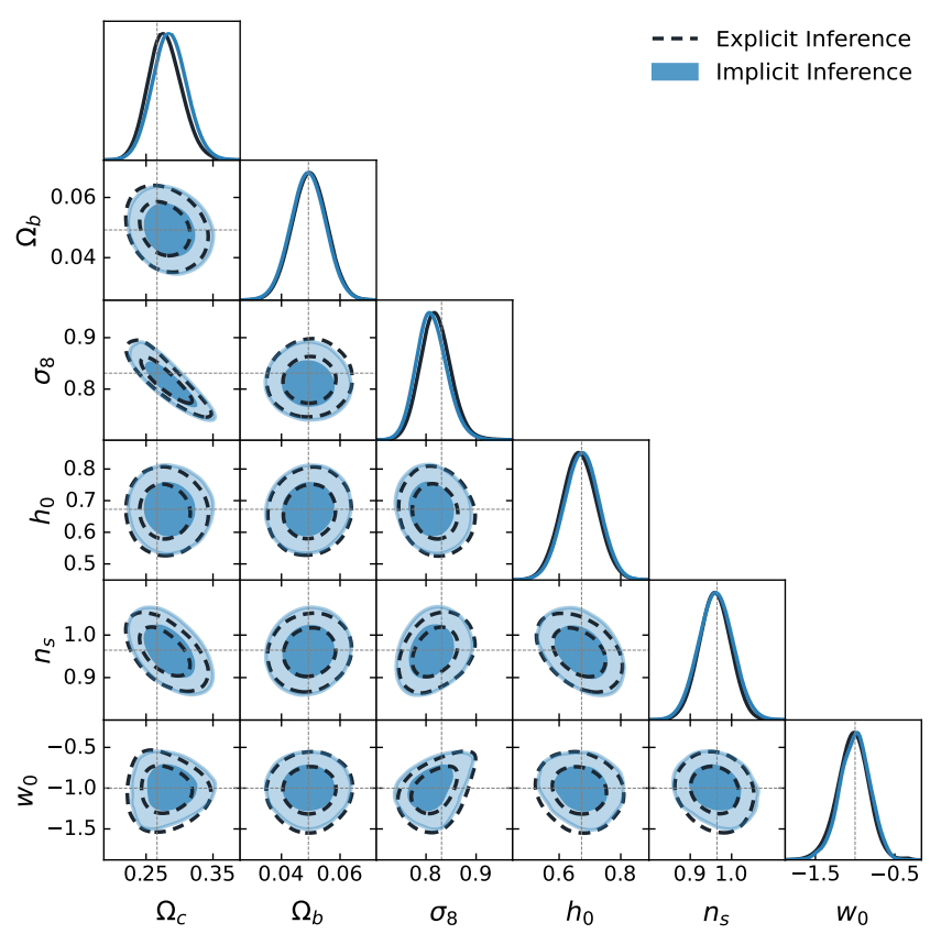
Implicit Inference is easier, cheaper, and yields the same results as Explicit Inference...
But Explicit Inference is cooler, so let's try to do it anyways!
Credit: Yuuki Omori, Chihway Chang, Justine Zeghal, EiffL
More seriously, Explicit Inference has some advantages:
- More introspectable results to identify systematics
- Allows for fitting parametric corrections/nuisances from data
- Provides validation of statistical inference with a different method
Challenges we will discuss in this talk
- Efficient Posterior Sampling
- Distributed and Differentiable Forward Models
- Fast Effective Modeling of Small Scales and Baryons
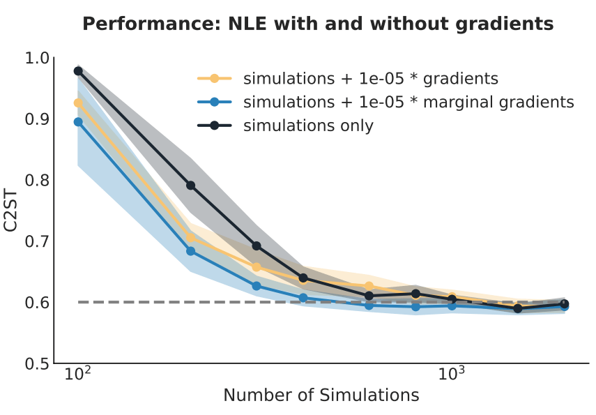
Benchmarking
Field-Level Explicit Inference
For Galaxy Redshift Surveys

Work led by Hugo Simon (CEA Paris-Saclay)
In collaboration with Arnaud de Mattia
<- On the job market! Don't miss out!
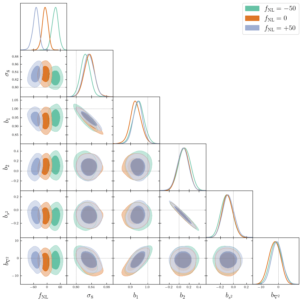
\(\Omega := \{ \Omega_m, \Omega_\Lambda, H_0, \sigma_8, f_\mathrm{NL},...\}\)

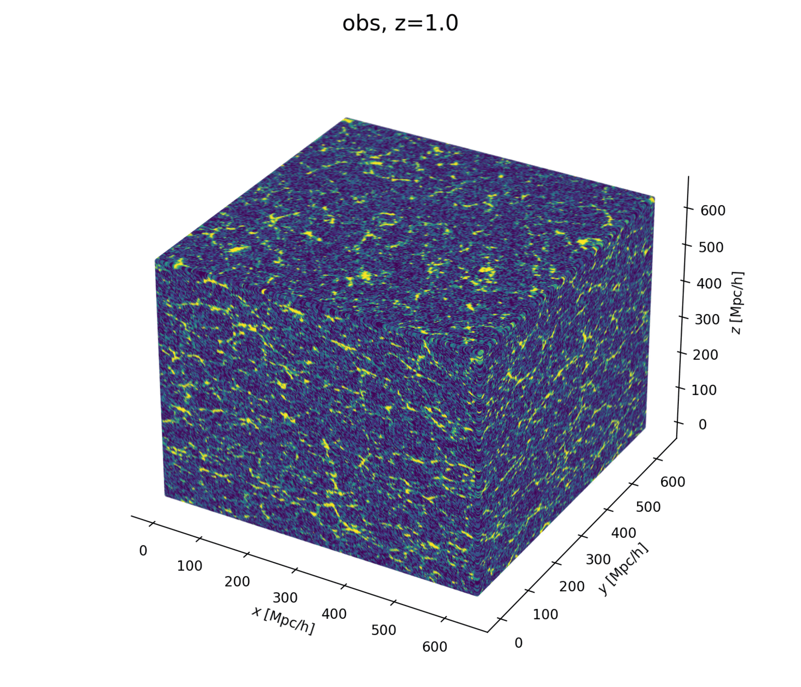
Linear matter spectrum
Structure growth
Cosmological Modeling and Inference
\(\Omega\)
\(\delta_L\)
\(\delta_g\)
inference
\(128^3\) PM on 8GPU:
4h MCLMC vs. \(\geq\) 80h HMC
-
Prior on
- Cosmology \(\Omega\)
- Initial field \(\delta_L\)
- EFT Lagrangian parameters \(b\)
(Dark matter-galaxy connection)
-
LSS formation: 2LPT or PM
(BullFrog or FastPM) - Apply galaxy bias
- Redshift-Space Distortions
- Observational noise
Modeling Assumptions


Fast and differentiable model thanks to (\(\texttt{NumPyro}\) and \(\texttt{JaxPM}\))
What Inference Looks Like
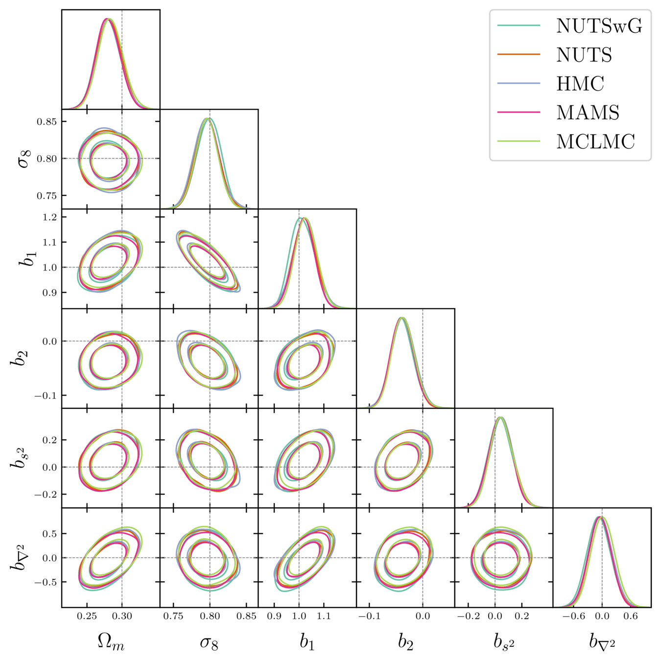
- Different samplers and strategies used for field-level (e.g. Lavaux+2018, Bayer+2023).
=> Additional comparisons required. - We provide a consistent benchmark for field-level from galaxy surveys. Build upon \(\texttt{NumPyro}\) and \(\texttt{BlackJAX}\).
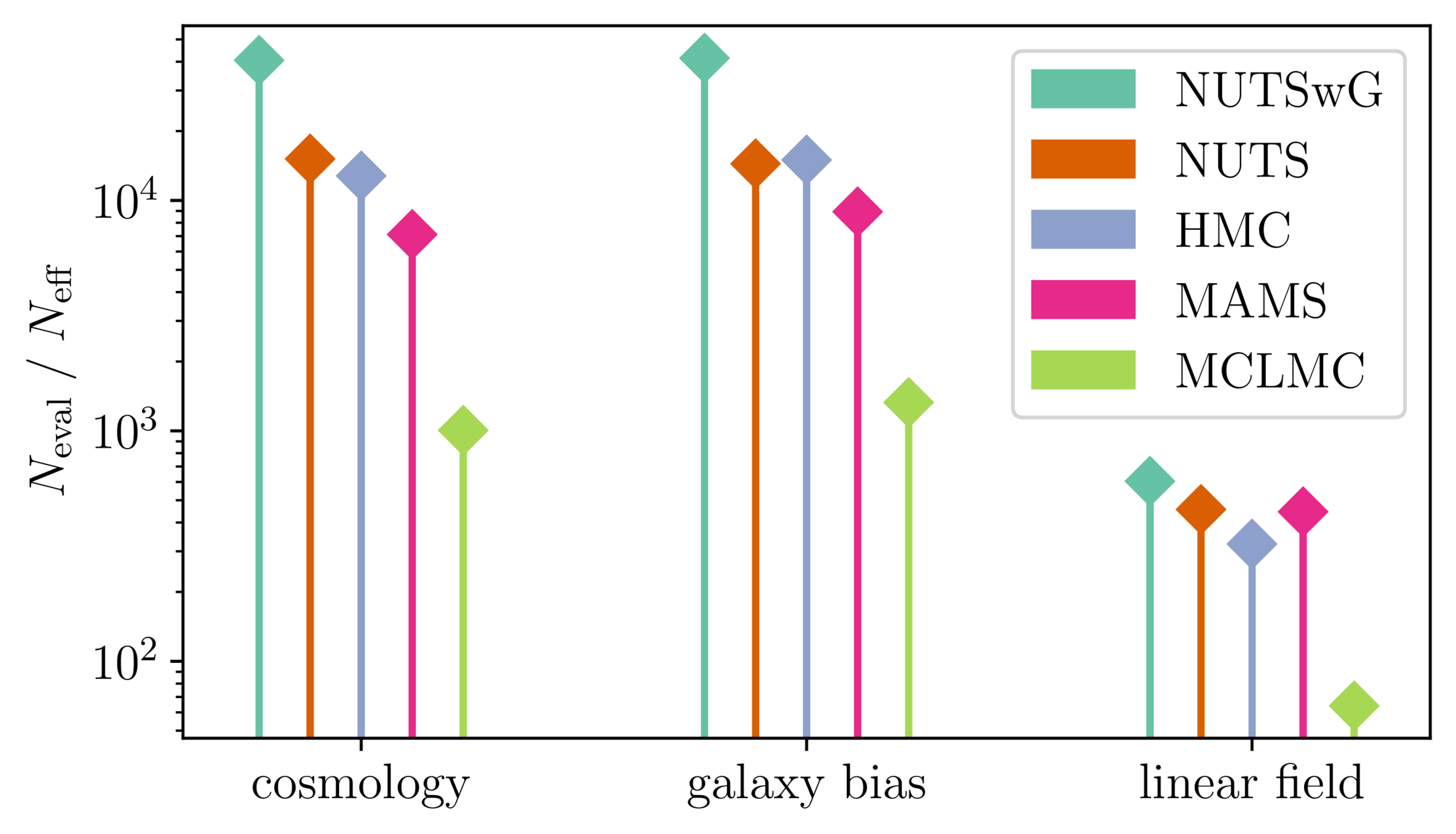
Samplers comparison
= NUTS within Gibbs
= auto-tuned HMC
= adjusted MCHMC
= unadjusted Langevin MCHMC
10 times less evaluations required
Unadjusted microcanonical sampler outperforms any adjusted sampler
Canonical/Microcanonical MCMC samplers
- \(\mathcal H(\boldsymbol q, \boldsymbol p) = \frac {\boldsymbol p^\top M^{-1} \boldsymbol p} {2 m(\boldsymbol q)} - \frac{m(\boldsymbol q)}{2} \quad ; \quad m=e^{-U/(d-1)}\)
- samples microcanonical/isokinetic ensemble $$\mathrm p_\text{C}(\boldsymbol q, \boldsymbol u) \propto \delta(H(\boldsymbol q, \boldsymbol u)) \propto \mathrm p (\boldsymbol q) \delta(|\boldsymbol u| - 1)$$
Hamiltonian Monte Carlo (e.g. Neal2011)
MicroCanonical HMC (Robnik+2022)
- \(\mathcal H(\boldsymbol q, \boldsymbol p) = U(\boldsymbol q) + \frac 1 2 \boldsymbol p^\top M^{-1} \boldsymbol p\)
- samples canonical ensemble $$\mathrm p_\text{C}(\boldsymbol q, \boldsymbol p) \propto e^{-\mathcal H(\boldsymbol q, \boldsymbol p)} \propto \mathrm p(\boldsymbol q)\,\mathcal N(\boldsymbol 0, M)$$
Will I Go to Jail for Using Unadjusted MCMC?
- Microcanonical dynamics \(\implies\) energy should not vary
- Numerical integration yields quantifiable errors that can be linked to bias
- Stepsize can be tuned to ensure controlled bias, see Robnik+2024
reducing stepsize rapidly brings bias under Monte Carlo error
Canonical MCMC samplers
Recipe😋 to sample from \(\mathrm p \propto e^{-U}\)
- take particle with position \(\boldsymbol q\), momentum \(\boldsymbol p\), mass matrix \(M\), and Hamiltonian $$\mathcal H(\boldsymbol q, \boldsymbol p) = U(\boldsymbol q) + \frac 1 2 \boldsymbol p^\top M^{-1} \boldsymbol p$$
- follow Hamiltonian dynamics during time \(L\)
$$\begin{cases} \dot {{\boldsymbol q}} = \partial_{\boldsymbol p}\mathcal H = M^{-1}{{\boldsymbol p}}\\ \dot {{\boldsymbol p}} = -\partial_{\boldsymbol q}\mathcal H = - \nabla U(\boldsymbol q) \end{cases}$$and refresh momentum \(\boldsymbol p \sim \mathcal N(\boldsymbol 0,M)\)
- usually, perform Metropolis adjustment
- this samples canonical ensemble $$\mathrm p_\text{C}(\boldsymbol q, \boldsymbol p) \propto e^{-\mathcal H(\boldsymbol q, \boldsymbol p)} \propto \mathrm p(\boldsymbol q)\,\mathcal N(\boldsymbol 0, M)$$
gradient guides particle toward high density sets
scales poorly with dimension
must average over all energy levels
Hamiltonian Monte Carlo (e.g. Neal2011)
Microcanonical MCMC samplers
Recipe😋 to sample from \(\mathrm p \propto e^{-U}\)
-
take particle with position \(\boldsymbol q\), momentum \(\boldsymbol p\), mass matrix \(M\), and Hamiltonian $$\mathcal H(\boldsymbol q, \boldsymbol p) = \frac {\boldsymbol p^\top M^{-1} \boldsymbol p} {2 m(\boldsymbol q)} - \frac{m(\boldsymbol q)}{2} \quad ; \quad m=e^{-U/(d-1)}$$
-
follow Hamiltonian dynamics during time \(L\)
$$\begin{cases} \dot{\boldsymbol q} = M^{-1/2} \boldsymbol u\\ \dot{\boldsymbol u} = -(I - \boldsymbol u \boldsymbol u^\top) M^{-1/2} \nabla U(\boldsymbol q) / (d-1) \end{cases}$$ and refresh \(\boldsymbol u \leftarrow \boldsymbol z/ \lvert \boldsymbol z \rvert \quad ; \quad \boldsymbol z \sim \mathcal N(\boldsymbol 0,I)\)
-
usually, perform Metropolis adjustment
- this samples microcanonical/isokinetic ensemble $$\mathrm p_\text{C}(\boldsymbol q, \boldsymbol u) \propto \delta(H(\boldsymbol q, \boldsymbol u)) \propto \mathrm p (\boldsymbol q) \delta(|\boldsymbol u| - 1)$$
single energy/speed level
let's try avoiding that
gradient guides particle toward high density sets
MicroCanonical HMC (Robnik+2022)
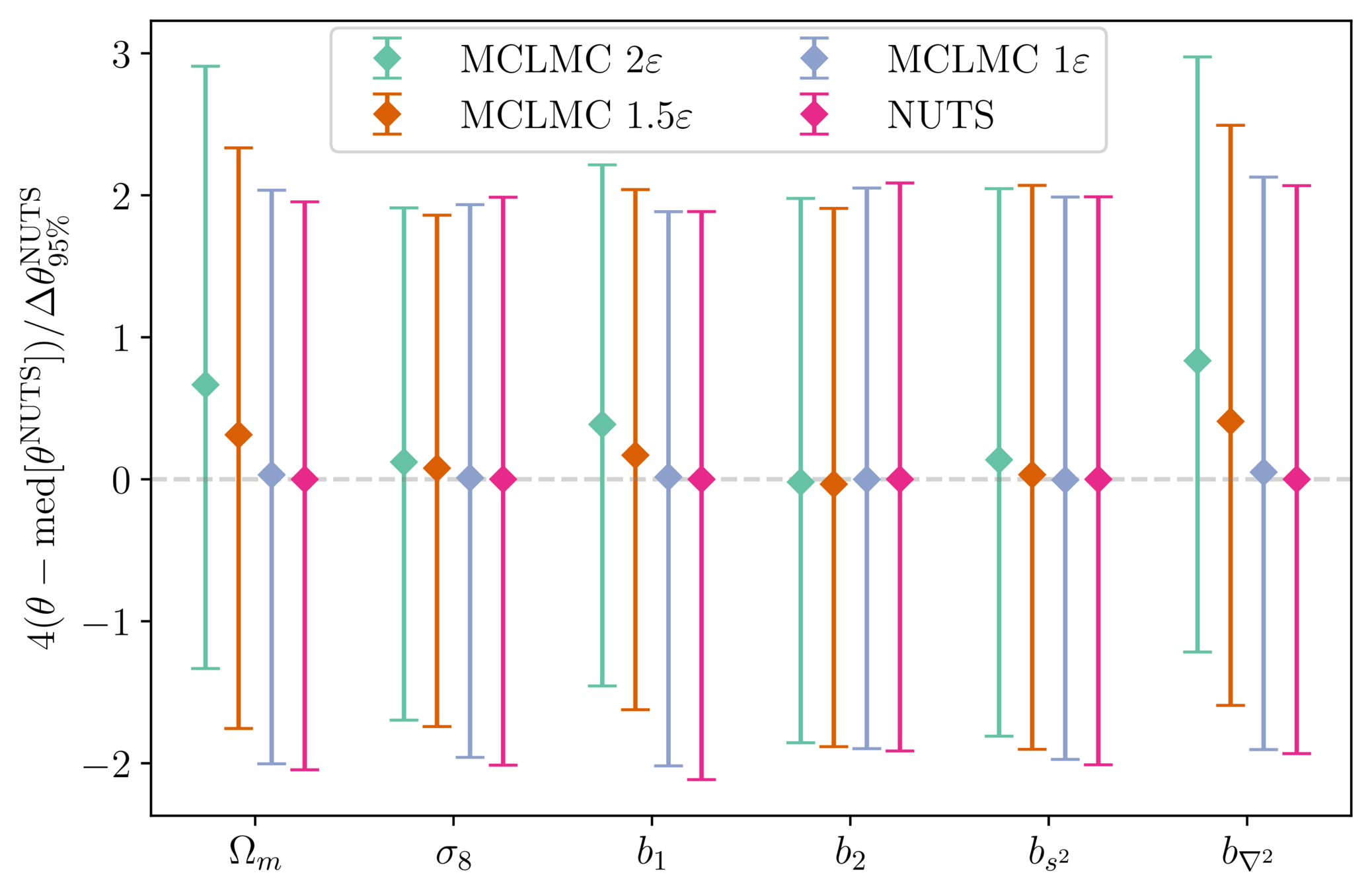
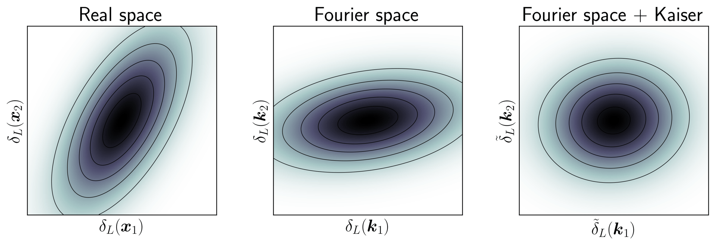
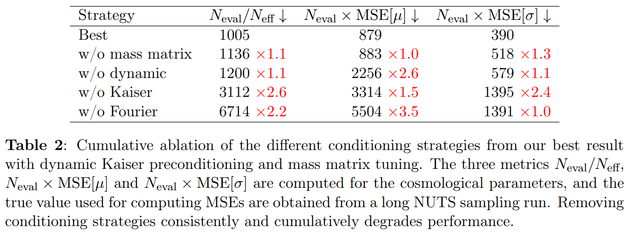
Impact of Preconditioning
- Sampling is easier when target density is isotropic Gaussian
- The model is reparametrized assuming a tractable Kaiser model:
linear growth + linear Eulerian bias + flat sky RSD + Gaussian noise
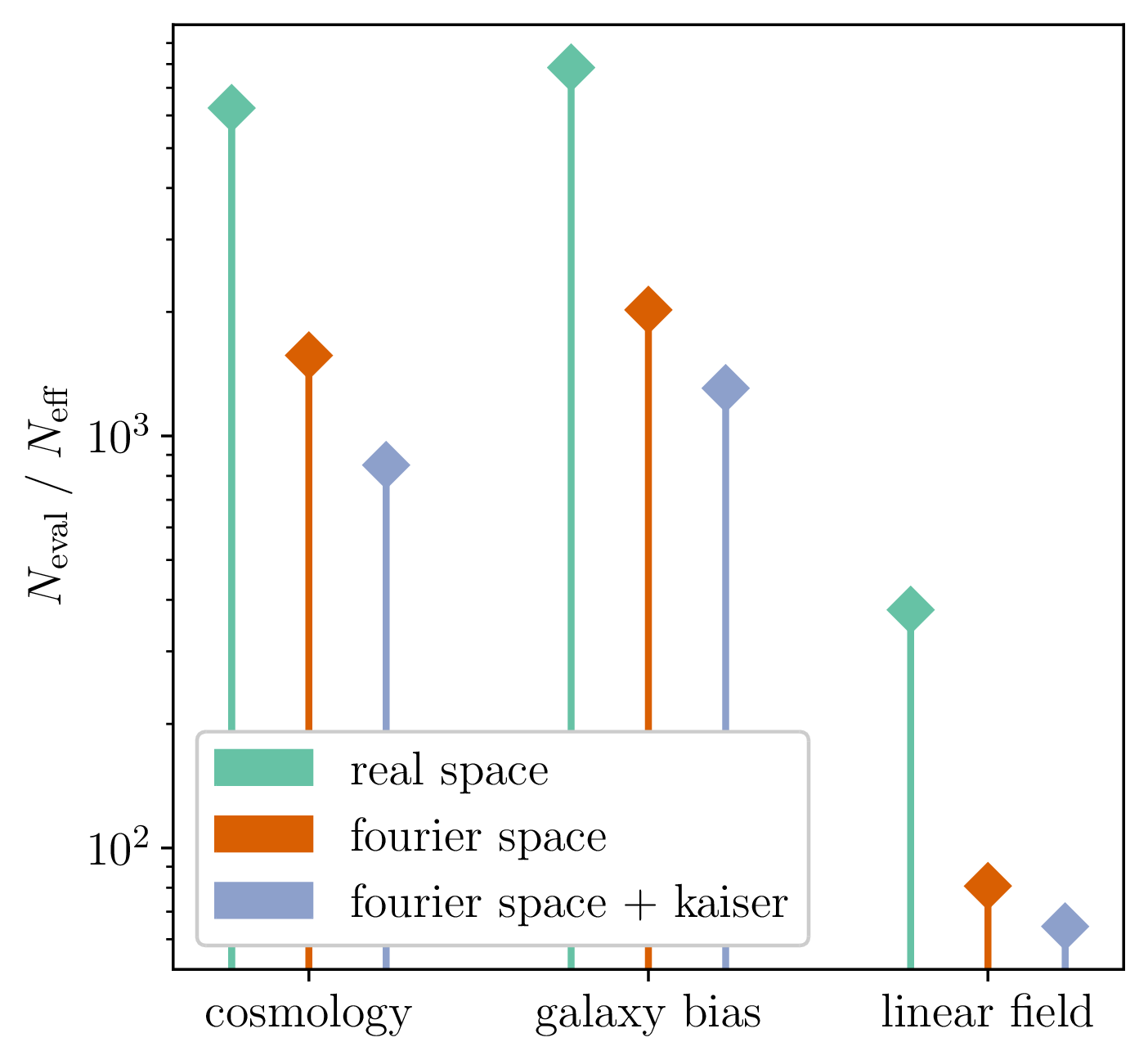
10 times less evaluations required
Impact of Resolution and Scale
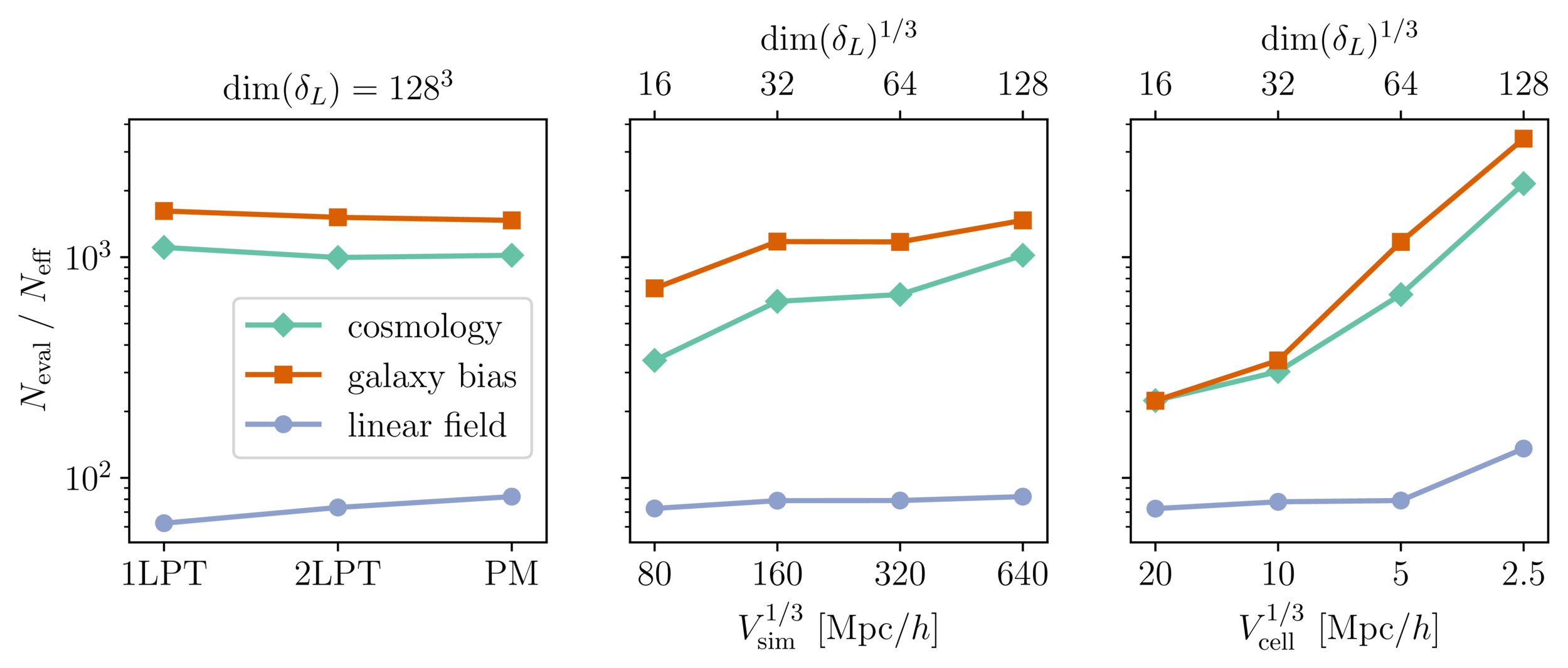
\(128^3\) PM on 8GPU:
4h MCLMC vs. \(\geq\)80h NUTS
Mildly dependent with respect to formation model and volume
Probing smaller scales could be harder
Distributed and Differentiable Cosmological Simulations
Work led by Wassim Kabalan (IN2P3/APC)
In collaboration with Alexandre Boucaud
<- On the job market! Don't miss out!
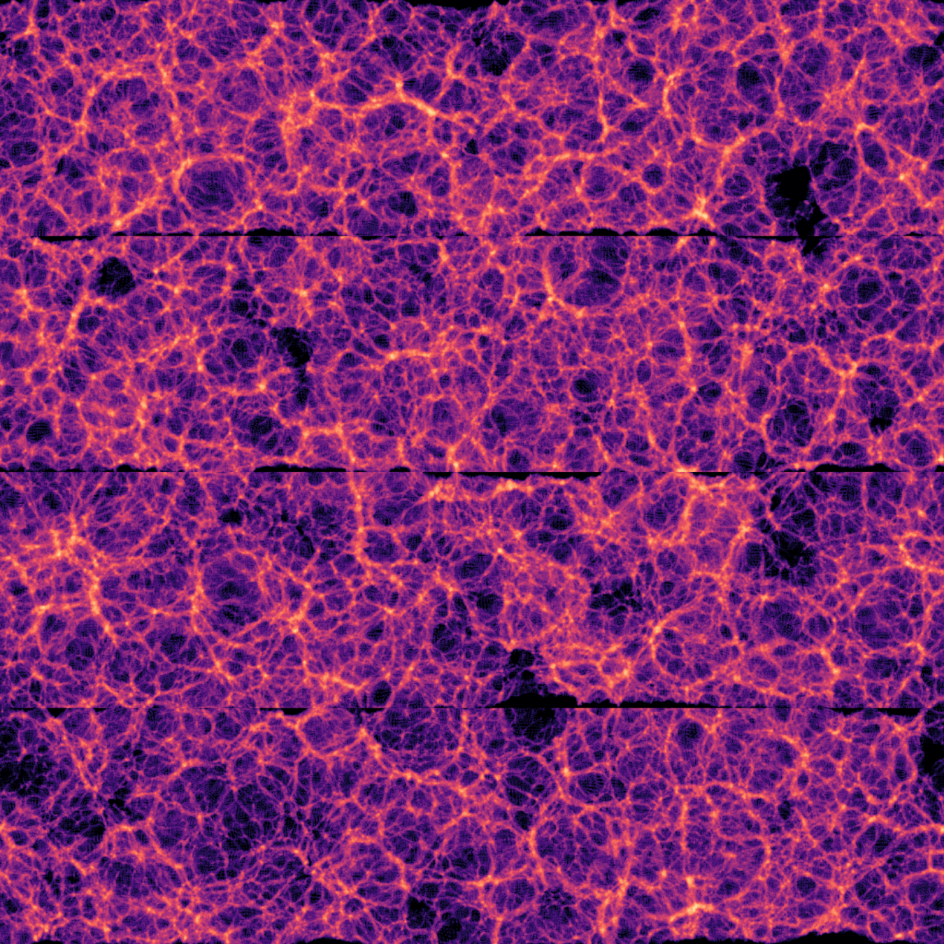
Weak Lensing requires significant resolution
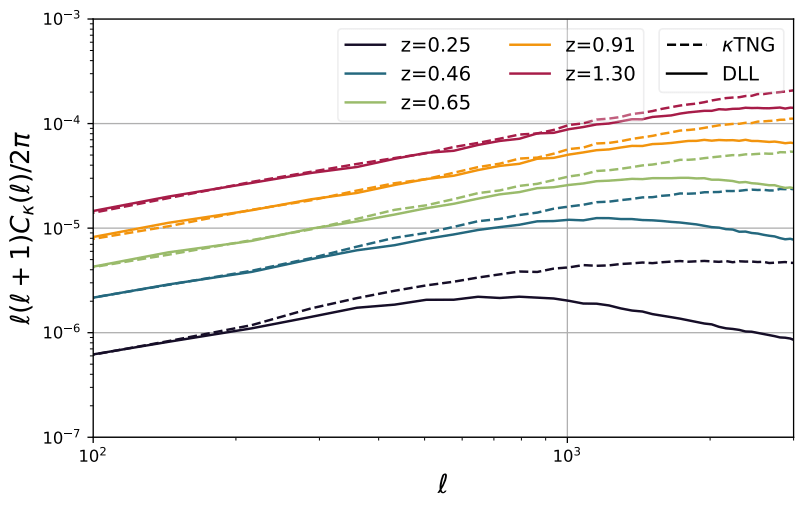
Differentiable Lensing Lightcone (DLL) - FlowPM
- 5 x 5 sq. deg. lensing field
- 205\(^3\) (\( h^{-1} \) Mpc)\(^3\) volume
- 128\(^3\) particles/voxels
=> Limit of what fits in a conventional GPU circa 2022

Towards JAX-based Differentiable HPC
- JAX v0.4.1 (Dec. 2022) has made a strong push for bringing automated parallelization and support multi-host GPU clusters!
- Scientific HPC still most likely requires dedicated high-performance ops
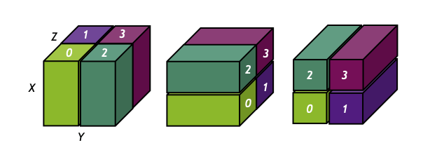
- JAX bindings to the high-performance cuDecomp (Romero et al. 2022) adaptive domain decomposition library.
- Provides parallel FFTs and halo-exchange operations.
- Supports variety of backends: CUDA-aware MPI, NVIDIA NCCL, NVIDIA NVSHMEM.


without halo exchange
with halo exchange
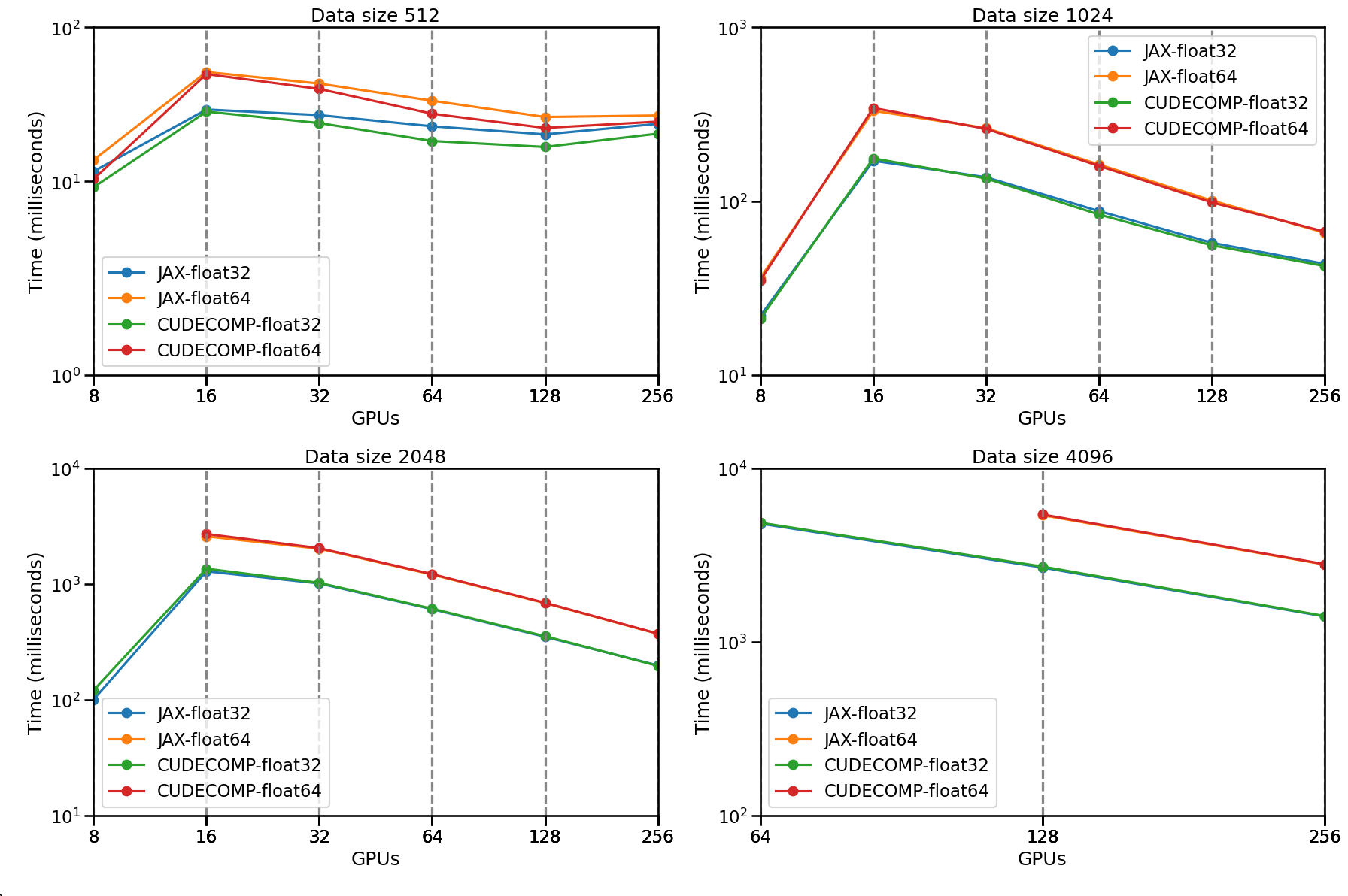
Strong Scaling Results
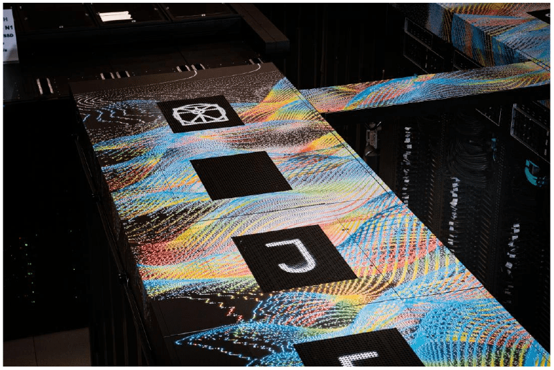

Jean Zay Supercomputer
JaxPM v0.1.6: Differentiable and Scalable Simulations
pip install jaxpm-
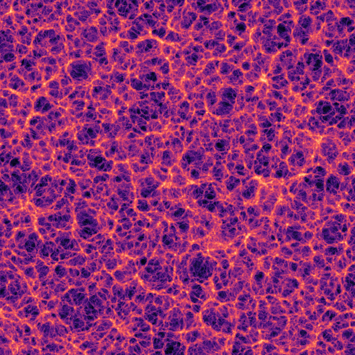
Multi-GPU and Multi-Node simulation with distributed domain decomposition (Successfully ran 2048³ on 256 GPUs), built on top of
jaxdecomp -
End-to-end differentiability, including force computation and interpolation
-
Compatible with a custom JAX compatible Reverse Adjoint solver for memory-efficient gradients (including Diffrax)
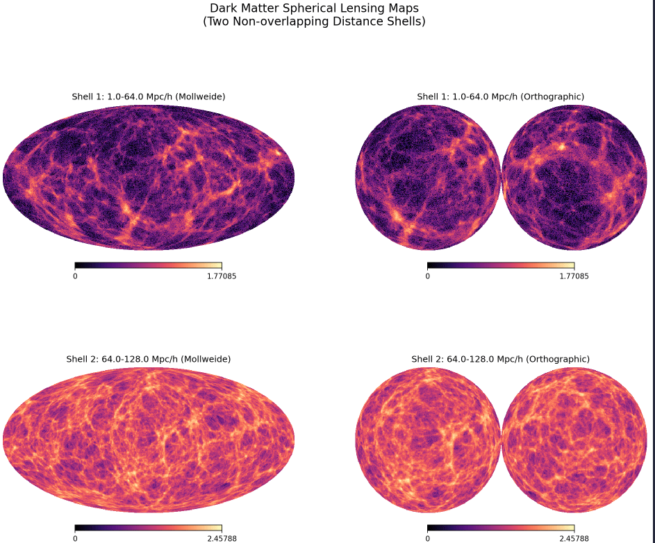
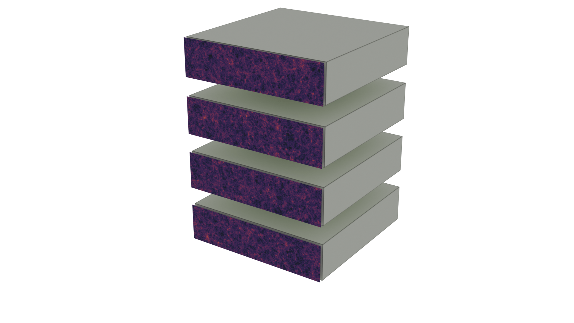
Under development: Full-Sky Differentiable Lensing Lightcones
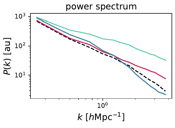
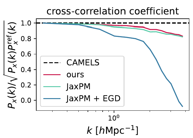
Hybrid Physical-Neural Simulator for Fast Cosmological Hydrodynamics
Work led by Arne Thomsen (ETH Zurich)
In collaboration with Tilman Troester, Chihway Chang, Yuuki Omori
Accepted at NeurIPS 2025 Workshop on Machine Learning for the Physical Sciences
Hybrid Physical-Neural Simulations
Dr. Denise Lanzieri
(now at Sony CSL)
CAMELS N-body
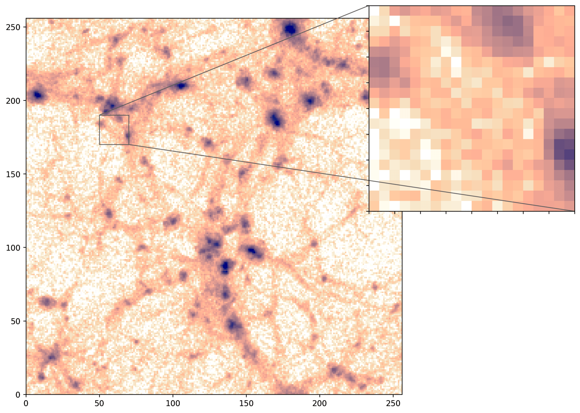
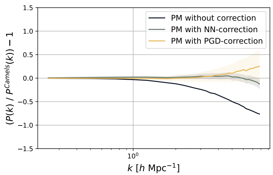
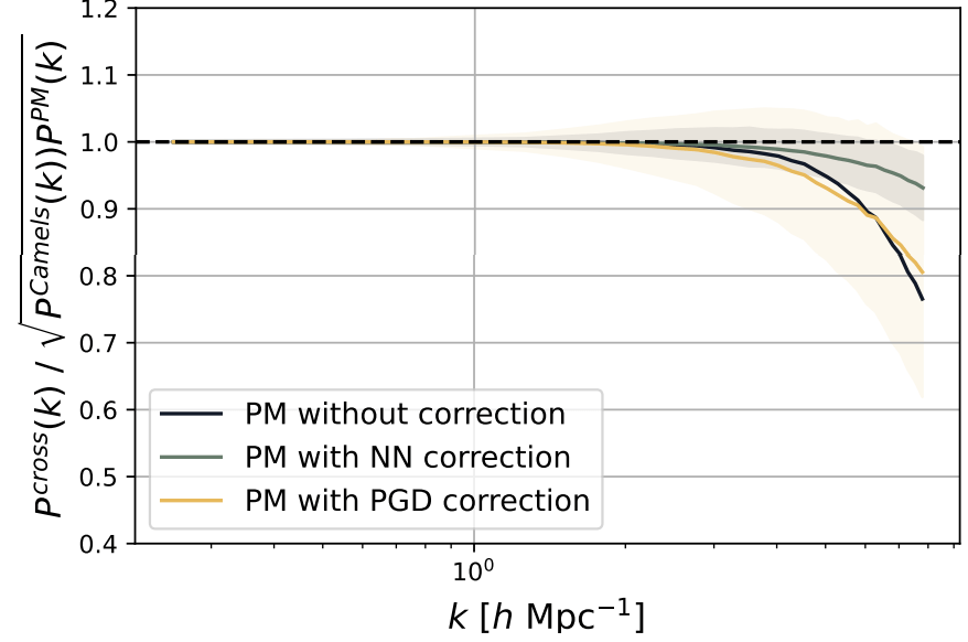
PM
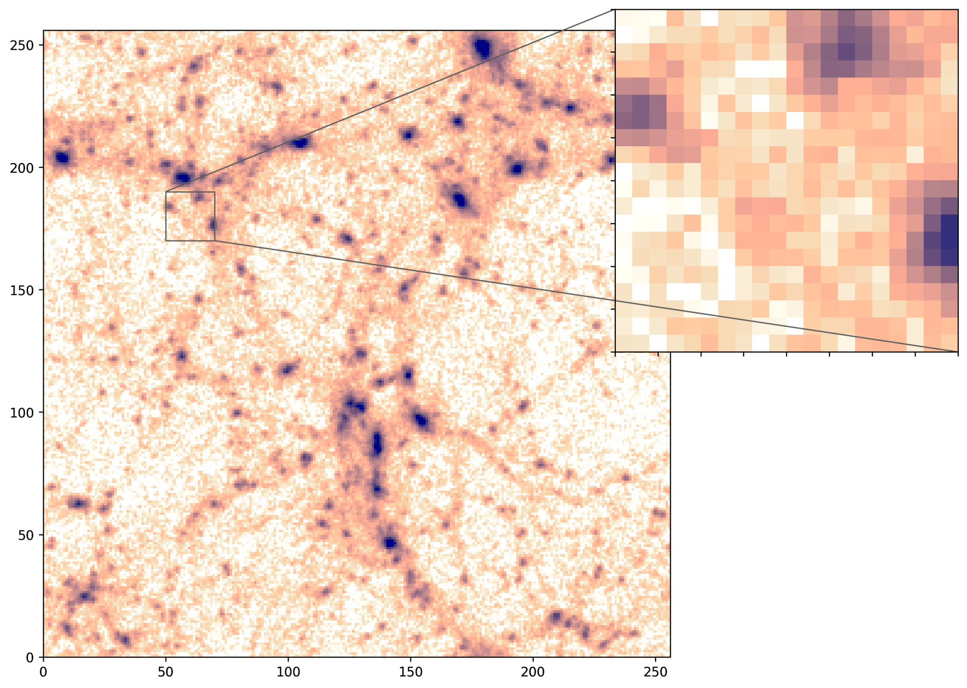
PM+NN
\left\{
\begin{array}{ll}
\frac{d \mathbf{x}}{d a} & = \frac{1}{a^3 E(a)} \mathbf{v} \\
\frac{d \mathbf{v}}{d a} & = \frac{1}{a^2 E(a)} F_\theta(\mathbf{x}, a), \\
F_\theta(\mathbf{x}, a) &= \frac{3 \Omega_m}{2} \nabla \left[ \phi_{PM} (\mathbf{x}) \ast \mathcal{F}^{-1} (1 + \color{#996699}{f_\theta(a,|\mathbf{k}|)}) \right]
\end{array}
\right.
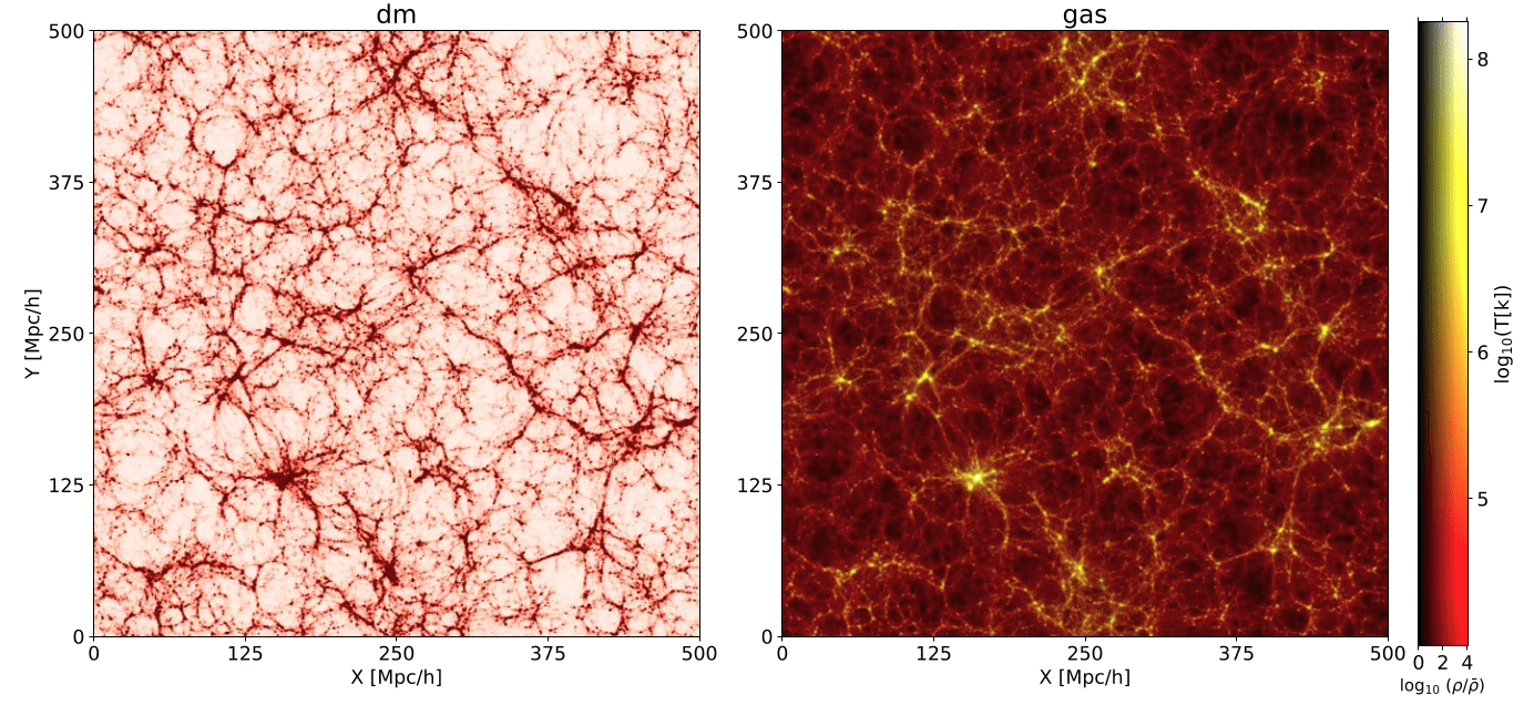
HYPER: Hydro-Particle-Mesh Code
\left\{
\begin{aligned}
\frac{d \mathbf{x}_{\mathrm{dm}}}{da} &= \frac{1}{a^{3} E(a)} \, \mathbf{v}_{\mathrm{dm}} \\
\frac{d \mathbf{v}_{\mathrm{dm}}}{da} &= -\frac{1}{a^{2} E(a)} \, \nabla \Phi_{\mathrm{tot}}
\end{aligned}
\right.
\qquad
\left\{
\begin{aligned}
\frac{d \mathbf{x}_{\mathrm{gas}}}{da} &= \frac{1}{a^{3} E(a)} \, \mathbf{v}_{\mathrm{gas}} \\
\frac{d \mathbf{v}_{\mathrm{gas}}}{da} &= -\frac{1}{a^{2} E(a)}
\left( \nabla \Phi_{\mathrm{tot}} + \frac{\nabla P}{\rho_{\mathrm{gas}}} \right)
\end{aligned}
\right.
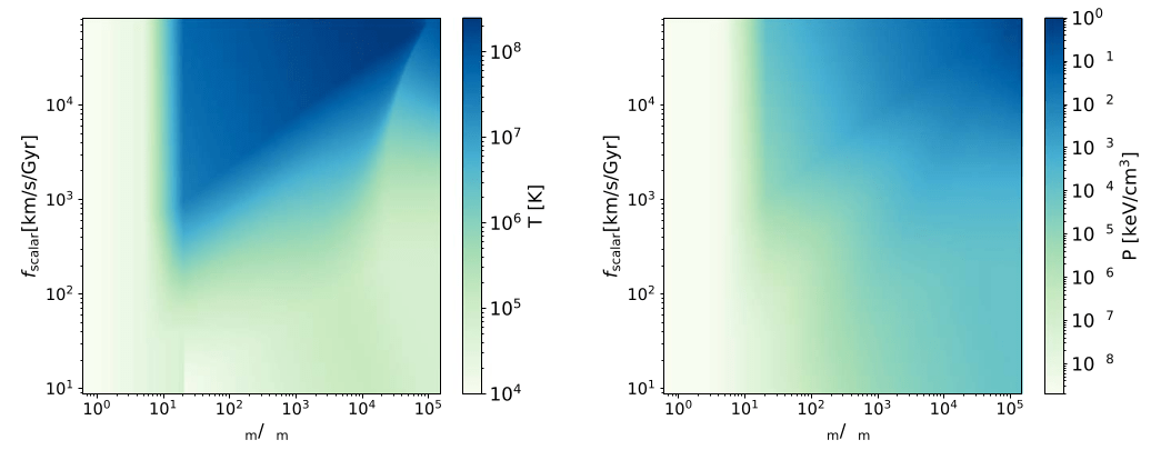
- HYPER proposes to use a halo model to compute \( P(M, r) \) analytically
- However, \( M \) and \( r \) are not available without halos, so HYPER uses a reparameterisation \( (M, r ) \rightarrow (\rho, f_{scalar}) \) which are trivially computed on a mesh
Neural Parameterization and Training
\left\{
\begin{aligned}
\frac{d \mathbf{x}_{\mathrm{dm}}}{da} &= \frac{1}{a^{3} E(a)} \, \mathbf{v}_{\mathrm{dm}} \\
\frac{d \mathbf{v}_{\mathrm{dm}}}{da} &= -\frac{1}{a^{2} E(a)} \, \nabla \Phi_{\mathrm{tot}}
\end{aligned}
\right.
\qquad
\left\{
\begin{aligned}
\frac{d \mathbf{x}_{\mathrm{gas}}}{da} &= \frac{1}{a^{3} E(a)} \, \mathbf{v}_{\mathrm{gas}} \\
\frac{d \mathbf{v}_{\mathrm{gas}}}{da} &= -\frac{1}{a^{2} E(a)}
\left( \nabla \Phi_{\mathrm{tot}} + \frac{\nabla P}{\rho_{\mathrm{gas}}} \right)
\end{aligned}
\right.
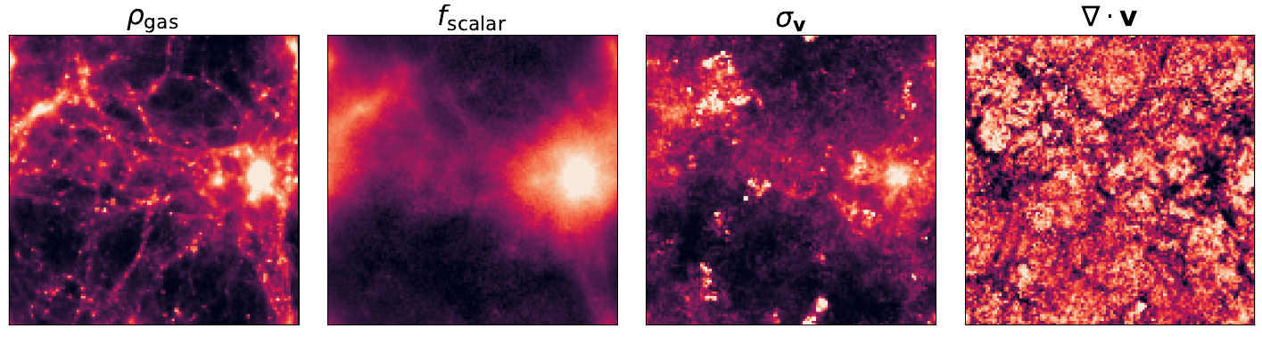
P_\theta (\mathbf{x}, a) = \rho_{gas} (\mathbf{x}) U_\theta (a, \rho, f_{scalar}, \sigma_v, \nabla \cdot v)
particle-wise multilayer perceptron
Neural Parameterization and Training
\left\{
\begin{aligned}
\frac{d \mathbf{x}_{\mathrm{dm}}}{da} &= \frac{1}{a^{3} E(a)} \, \mathbf{v}_{\mathrm{dm}} \\
\frac{d \mathbf{v}_{\mathrm{dm}}}{da} &= -\frac{1}{a^{2} E(a)} \, \nabla \Phi_{\mathrm{tot}}
\end{aligned}
\right.
\qquad
\left\{
\begin{aligned}
\frac{d \mathbf{x}_{\mathrm{gas}}}{da} &= \frac{1}{a^{3} E(a)} \, \mathbf{v}_{\mathrm{gas}} \\
\frac{d \mathbf{v}_{\mathrm{gas}}}{da} &= -\frac{1}{a^{2} E(a)}
\left( \nabla \Phi_{\mathrm{tot}} + \frac{\nabla P}{\rho_{\mathrm{gas}}} \right)
\end{aligned}
\right.
\mathcal{L} = \sum_{s} \left[
H(\mathbf{x}_{s} - \mathbf{x}_{s}^{\mathrm{ref}} )
+ \lambda H \bigl(\mathbf{v}_{s} - \mathbf{v}_{s}^{\mathrm{ref}}\bigr)
+ \mu \left\| \frac{P_{s}(|\mathbf{k}|)}{P_{s}^{\mathrm{ref}}(|\mathbf{k}|)} - 1 \right\|_{2}^{2}
\right]
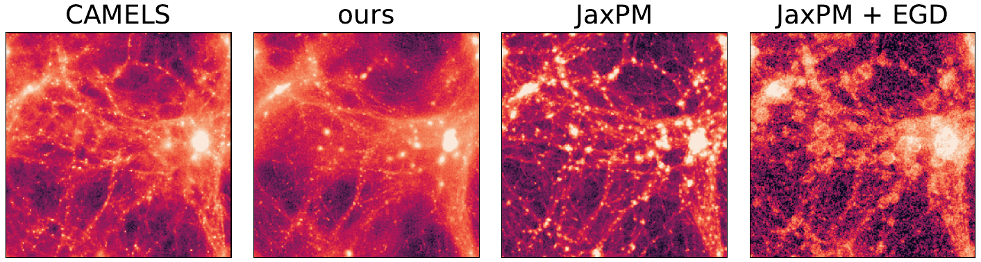
\rho_{gas}
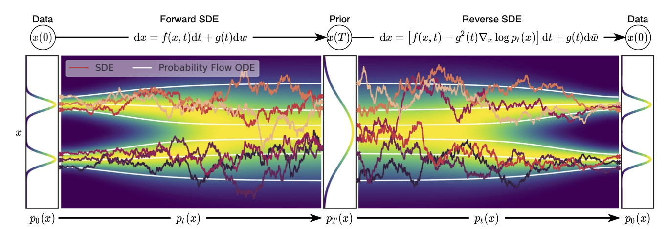
Fun project this week (discussing with Carol): Hybrid physical-neural SDE

dX_a \;=\; \Big[ f_H\!\big(X_a, a\big) \;+\; r_\theta\!\big(X_a, a\big) \Big]\, da
\;+\; B_\theta(a)\, dW_a ,
Just food for thought, not a full project
Concluding Thoughts
Interesting things to think about...
- Coordinated Development of a JAX-based Ecosystem
- We could imagine interoperable and independent components (module for cosmology, module for PM operations, module for solver, ...)
- We could imagine interoperable and independent components (module for cosmology, module for PM operations, module for solver, ...)
- Standardization and Parametrization of Fast Hybrid models
- We could imagine setting standards for effective models, fitted on various simulations, to provide a library of small scale/baryon models
- We could imagine setting standards for effective models, fitted on various simulations, to provide a library of small scale/baryon models
- Proper and Reproducible Sampling / Inference Benchmarking
- We could imagine extending Hugo's work and build a live and reproducible leaderboard.
Differentiable Forward Models and Efficient Sampling
By eiffl
Differentiable Forward Models and Efficient Sampling
Putting the Cosmic Large-scale Structure on the Map: Theory Meets Numerics


