MERCS
Versatile models with decision trees
ADS second oral presentation
January 20, 2020

Overview
- Introduction to MERCS
- Predictions with MERCS
- Anomaly detection with MERCS
- Administration
1. Introduction to MERCS
Motivation
A typical ML model can solve this
Given
what's the value of ?
X
Y
- Idealized scenario: if you do not know the exact task on beforehand, this paradigm breaks down.
- E.g.: anomaly detection (e.g. on sensor data), prediction in spreadsheets, ...
Disadvantage
Motivation
- You can cope with missing values
- You can switch targets
- You can switch the amount of targets
Advantages
Given
what's the value of ?
X
Y
A versatile ML model can solve this.
versatile
Example of a versatile model
Bayesian network
A
B
C
A
B
C
A
B
C
Compute distribution
of C, given A and B
A
B
C
Example of a versatile model
Bayesian network
A
B
C
A
B
C
- Compute distribution of B, given A.
- Compute C, given A and the distribution over B.
Example of a versatile model
Bayesian network
A
B
C
A
B
C
ADVANTAGES
DISADVANTAGES
Fully interpretable and completely versatile
Scalability: structure learning and inference are hard problems.
Works best on nominal data, handling numeric data is non-trivial.
Example of a versatile model
Bayesian network
Versatile models comparison
PGM
kNN
NN
Nominal + Numeric data
Interpretable
Scalable
Our solution
WHAT?
WHY?
HOW?
A multi-directional ensemble of decision trees could be a versatile model.
DTs are fast, interpretable, handle nominal and numeric attributes, ensembles are trivial to parallellize, ...
A minor modification of the Random Forest paradigm: allow for randomness in the target attributes.
Our solution
HOW?
A minor modification of the Random Forest paradigm: allow for randomness in the target attributes.
RF(X, Y) = \{T_{X_i \rightarrow Y} | X_i \subseteq X \land
X_i \cap Y = \emptyset \}
M(A) = \{T_{X_i \rightarrow Y_i} | X_i \subseteq A \, \land
Y_i \subseteq A \, \land
X_i \cap Y_i = \emptyset \}
Our solution
f_1:
X
\rightarrow
Y
Standard ML-model
Our solution
f_1:
X
\rightarrow
Y
f_2:
X
\rightarrow
Y
f_3:
X
\rightarrow
Y
MERCS model
Compact representation:
f_1
f_2
f_3:
f_3
Versatile models comparison
PGM
kNN
NN
Nominal + Numeric data
Interpretable
Scalable
MERCS
Versatile models comparison
PGM
kNN
NN
Nominal + Numeric data
Interpretable
Scalable
MERCS
Learning
Prediction
Results
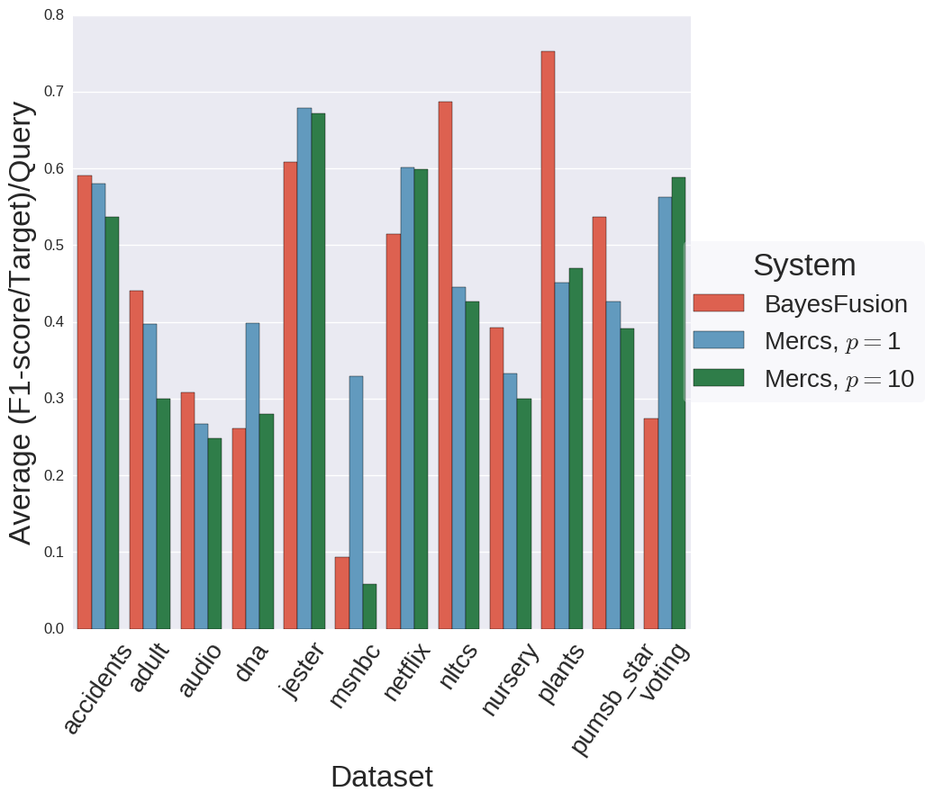
Competitive predictive performance when compared to PGMs
Results
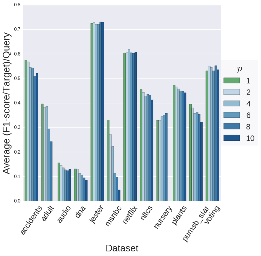
Multi-target trees can reduce the training time whilst maintaining performance.
Results
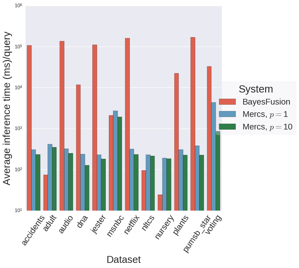
Inference is orders of magnitude faster in MERCS when compared to PGMs
Summary
- Introduced a first prototype of our MERCS system
- Experimental evaluation showed competitive predictive performance + large speedup at prediction time.
2. Predictions in MERCS
Problem
MERCS should handle any prediction task
- At training time: prediction task unknown
- At prediction time: you do not have the 'perfect' tree at your disposal
- Prediction algorithms overcome this discrepancy
MERCS MODEL
f_1
f_2
f_3
QUERIES
q_1
q_2
q_3
Problem
MERCS should handle any prediction task
- At training time: prediction task unknown
- At prediction time: you do not have the 'perfect' tree at your disposal
- Prediction algorithms overcome this discrepancy
2 main ideas
attribute
importance
chaining
Attribute Importance
PROBLEM
ASSUMPTION
IDEA
TRADEOFF
Which trees to use?
Trees with many missing inputs are likely to be mistaken.
Attribute Importance can quantify this effect.
Many trees vs. Good trees
Attribute Importance
IDEA
DEFINITION
CRITERION
Attribute importance is a way to quantify how appropriate a given tree is
I(A_j, T^i) \propto \sum \, p(\tau) \cdot \Delta i(\tau, A_j)
\{\tau|\tau \in T^i, a(\tau) = A_j\}
C(T_{X^i \rightarrow Y^i}) \propto \sum I(A_j, T^i)
\{A_j | A_j \in X^i \cap X^q\}
Cf. Louppe et al., Understanding variable importances in forests of randomized trees, NeurIPS 2013
...or the original CART manual
Attribute Importance

Baseline (RF)
Most-relevant attribute importance
Query:
\{A_1, A_3\} \rightarrow \{A_4\}
Chaining
PROBLEM
ASSUMPTION
IDEA
TRADEOFF
Which trees to use?
Missing inputs are also predictable with MERCS itself
Chaining of component trees to answer a given query
Bottom-up vs. Top-Down
Cf. Read et al., Classifier chains for multi-label classification, ECMLPKDD 2009
Chaining

Bottom-Up Chaining
Query:
\{A_1, A_2\} \rightarrow \{A_3\}
Top-Down Chaining
Chaining
Bottom-Up Chaining
Query:
\{A_1, A_2\} \rightarrow \{A_3\}
Use most appropriate models, given
\{A_1, A_2\}
Use most appropriate models, given
\{A_1, A_2, A_4\}
Chaining
Bottom-Up Chaining
Query:
\{A_1, A_2\} \rightarrow \{A_3\}
Top-Down Chaining
Chaining
Query:
\{A_1, A_2\} \rightarrow \{A_3\}
Use most appropriate models, for target
\{A_4\}
Use most appropriate models, for target
\{A_3\}
Top-Down Chaining
Results
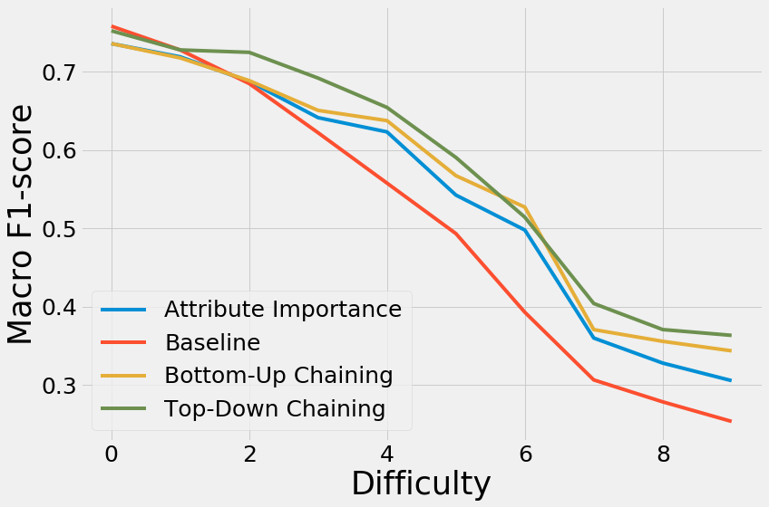
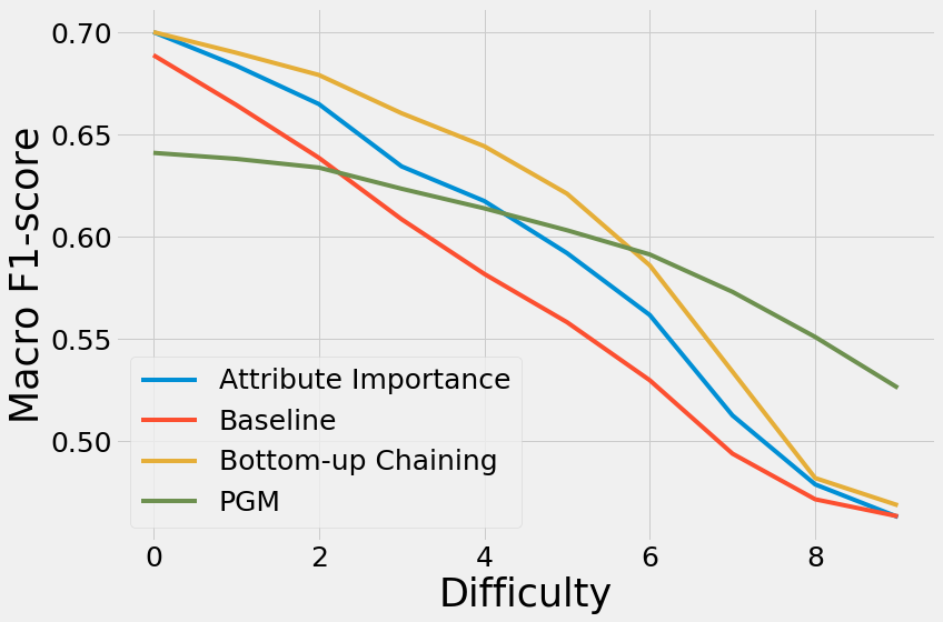
- Attribute Importance works
- Both chaining methods are beneficial
- With many missing values, the methods converge again
Results
- PGMs are more robust with respect to missing values
- Baseline MERCS: at ~20% missing values, PGM do better
- MERCS with chaining: this point moves to ~60% of missing values!
Summary
Reasonable amount of missing values (<50%) Chaining really works
General approach for MD-ensembles
Obvious costs at prediction time
With too many attributes missing, every tree is flawed and no prediction algorithm can solve that.
3. Anomaly detection with MERCS
An anomaly detector based on many predictive functions, a MERCS model.
Detection of an anomaly is only step one,
ideally we can understand, and ultimately prevent anomalies
A MERCS model splits the dataset in many 'contextual subpopulations'.
We then detect
A) anomalous subpopulations
B) anomalies within subpopulations.
WHY?
WHAT?
HOW?
Introduction
'contextual subpopulations'
Contextual Subpopulation
WHAT?
WHY?
HOW?
A subpopulation where all instances share a common context.
Anomalies are context-dependent.
Each node in a decision tree automatically represents such a subpopulation.
Contextual Subpopulation
P
B
R
M
F
Imagine a database of people (P)
Which contains basketball players (B) and regular persons (R)
And those basketball-players are both male (M) and female (F)
Contextual Subpopulation
P
B
R
M
F
This decision tree predicts the height of the persons in the database.
Example 01
Say, $$h=210 \,cm$$
Whether or not this is anomalous depends on context.
In R, probably yes.
In M, probably not.
Contextual Subpopulation
P
B
R
M
F
This decision tree predicts the height of the persons in the database.
Example 02
Say, $$h=165 \,cm$$
Whether or not this is anomalous depends on context.
In M, probably yes.
In R, probably not.
Contextual Subpopulation
P
B
R
M
F
This decision tree predicts the height of the persons in the database.
Anomaly Detection Mechanism 01
Model each contextual subpopulation by a density estimation to detect anomalies within such a subpopulation.
- 1D-density estimation on the target attribute of the decision tree.
Contextual Subpopulation
P
B
R
M
F
This decision tree predicts the height of the persons in the database.
Example 03
Assume that $$ |R| = 3,$$
Despite the fact that R is modelled well, it is the odd one out.
In a database of basketball players, these are 'anomalies'.
Contextual Subpopulation
P
B
R
M
F
We define a distance metric between different subpopulations in order to detect anomalous subpopulations.
- LOF with a slightly modified distance metric.
Anomaly Detection Mechanism 02
Summary
- MERCS provides a set of contextual subpopulations
- Anomalies inside subpopulations are discovered via density estimation in the target attribute
- Anomalous subpopulations are discovered through LOF
4. Administration
Administration
TEACHING
THESIS
BRI (4 times)
DB (4 times)
Supervised 7 theses so far, 2 in progress. (+ one best thesis award)
ADS
2 ECTS in transferable skills: OK
3 ECTS in DTAI seminar
Big Data Winterschool
Teaching Assistant Training: OK
Scientific Integrity: OK
Administration
PUBLICATIONS

Thank you
ADS-overview II
By eliavw
ADS-overview II
ADS Overview Presentation


