Optimization is everywhere: machine learning, operation research, data mining, theoretical computer science, etc.

\underset{x \in C}{\min} ~f(x)

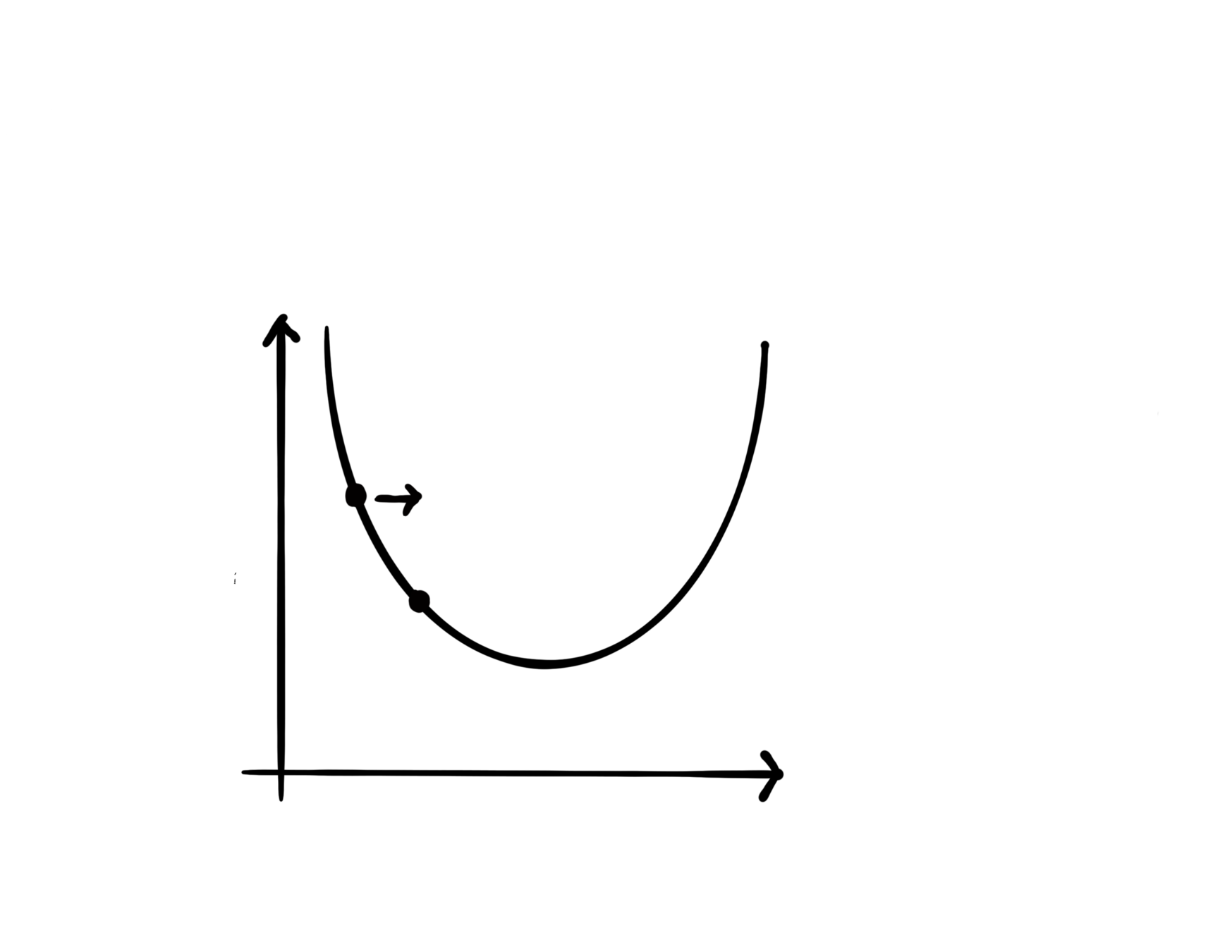
First-order methods:

x^{(t)} = \text{span}\{ x^{(0)}, \nabla f( x^{(0)} ), \nabla f( x^{(1)} ), \ldots, \nabla f( x^{(t-1)} ) \}

Why first-order methods?

Background and motivation

x^{(t)}

x^{(t+1)}

The literature

Gradient descent can be traced back to Cauchy's work in1847.

It is gaining increasing interest in the past 3 decades due to its empirical success.

Fundamental works have been done by pioneering researchers (Bertsekas, Nesterov, etc.).

There are still gaps between theory and practice.

Coordinate optimization

Mrrior descent

Stochastic subgradient method

Coordinate Optimization

Coordinate Descent

For

t = 0, 1, 2, \ldots,

Select coordinate

i \in [d]

Update

x_i^{(t+1)} = x_i^{(t)} - \eta_t \nabla_i f( x^{(t)} )

Different coordinate selection rules:

Random selection:

Cyclic selection:

Random permuted cyclic (the matrix AMGM inequality conjecture is false [LL20, S20])

Greedy selection (Gauss-Southwell)

i \in \arg\max_{ j \in [d] } | \nabla_j f( x^{(t)} ) |

i \sim \mathrm{uniform}\{1,2,\ldots, d\}

i = (t-1) ~\mathrm{mod}~ d + 1

GCD for Sparse Optimization

\underset{ x \in \mathbb{R}^d }{\min}~F(x) \coloneqq f(x) + g(x)

regularizer

One-norm regularization or nonnegative constraint can promote a sparse solution.

When initailzed at zero, greedy CD is observed to have an implicit screening ability to select variables that are nonzero at solution.

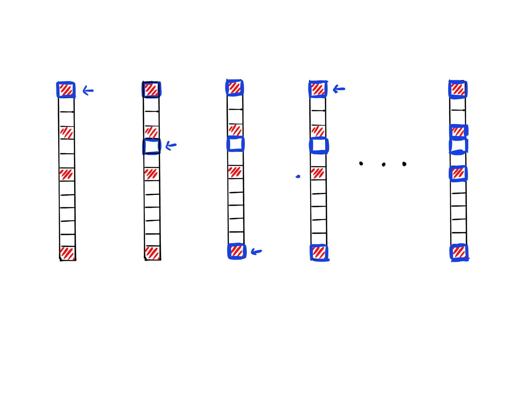
Iter 1

Iter 2

Iter 3

Iter 4

Iter

T

g(x) = \lambda \| x \|_1

g(x) = \delta_{\geq 0}(x)

data fitting

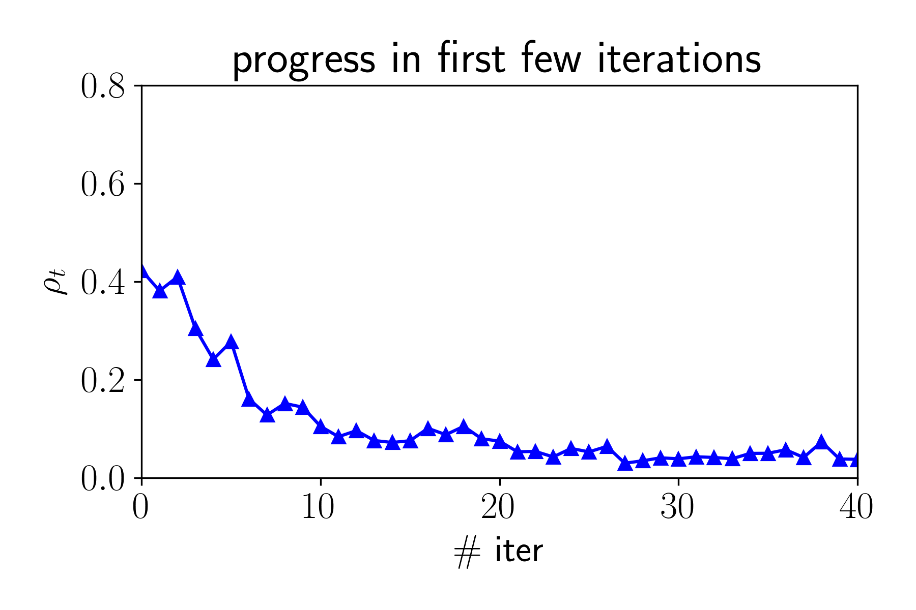
GCD for Sparse Optimization

[FFSF, AISTATS'20]

We provide a theoretical characterization of GCD's screening ability:

GCD converges fast in first few iterations.

The iterate is "close" the to solution when the iterate is still sparse, and sparsity pattern will not further expand anymore.

x^{(0)}

x^{*}

x^{(100)}

d = 10^4, \| x^* \|_0 = 10

\| x^{(t)} \|_0 \leq 110

for

t > 100

\delta

From coordinate to atom

Learning a sparse representation of an atomic set :

\mathcal{A}

x^* = \sum_{a \in \mathcal{A}} c_a a

such that

c_a \geq 0~\forall a \in \mathcal{A}

sparse vector:

\mathcal{A} = \{ \pm e_1, \pm e_2, \ldots, \pm e_d \}

Low-rank matrix:

\mathcal{A} = \{ uv^T \mid u \in \mathbb{R}^{n}, v \in \mathbb{R}^m, \|u\| = \|v\| = 1 \}

Our contribution: how to identify the atoms with nonzero coefficients at solution during the optimization process.

[FFF21] Submitted

Online Mirror Descent

Online Convex Optimization

Play a game for rounds, for

T

Propose a point

x^{(t)} \in \mathcal{X}.

Suffer loss

f_t( x^{(t)} ).

t = 1,2,\ldots, T

The goal of online learning algorithm: obtain sublinear regret

\displaystyle \mathrm{Regret} (T, z) \coloneqq \sum_{t=1}^T f_t( x^{(t)} ) - \sum_{t=1}^T f_t(z).

\mathrm{Regret} (T, z) = o(T) \to \mathrm{Regret} (T, z)/T \to 0.

player's loss

competitor's loss

Mirror Descent (MD) and Dual Averaging (DA)

MD and DA are parameterized by mirror map, they have advantages over the vanilla projected subgradient method.

f_t(x) = c_t^T x \quad \text{and} \quad \mathcal{X} = \left\{ \sum_{i=1}^d x_i = 1, x_i \geq 0 \right\}, ~\|c_t\|_{\infty} \leq 1.

When is known in advance or , both MD and DA guarantee regret

T

\mathcal{O}( \sqrt{T} ).

When is unknown in advance and , then MD has rate while DA still guarantees regret.

T

\sup_{x, y \in \mathcal{X}} D_\Phi(x, y) = +\infty

\Omega ( T )

\mathcal{O}( \sqrt{T} )

\sup_{x, y \in \mathcal{X}} D_\Phi(x, y) < +\infty

Our contribution: fix the divergence issue of MD and obtain

regret.

\mathcal{O}( \sqrt{T} )

OMD Algorithm

[FHPF, ICML'20]

Primal

Dual

x^{(t)}

\hat{x}^{(t)}

\nabla \Phi

\hat{y}^{(t)}

-\eta_t \nabla f_t( x^{(t)} )

y^{(t)}

x^{(t+1)}

Bregman projection

\nabla \Phi^*

Figure accredited to Victor Portella

Stabilized OMD

[FHPF, ICML'20]

Primal

Dual

x^{(t)}

\hat{x}^{(t)}

\nabla \Phi

\hat{y}^{(t)}

-\eta_t \nabla f_t( x^{(t)} )

y^{(t)}

x^{(t+1)}

Bregman projection

\nabla \Phi^*

\hat{x}^{(0)}

\hat{w}^{(t)}

}

\gamma_t

With stabilization, OMD can obtain regret.

\mathcal{O}( \sqrt{T} )

(Stochastic) Subgradient Method

Smooth v.s. Nonsmooth Minimization

Consider minimizing a convex function

The iteration complexity of gradient descent (GD) and subgradient descent (subGD) for smooth and nonsmooth objectives:

\underset{ x \in \mathbb{R}^d }{\min}~ f(x).

when is smooth:

f

\mathcal{O}(1/\epsilon).

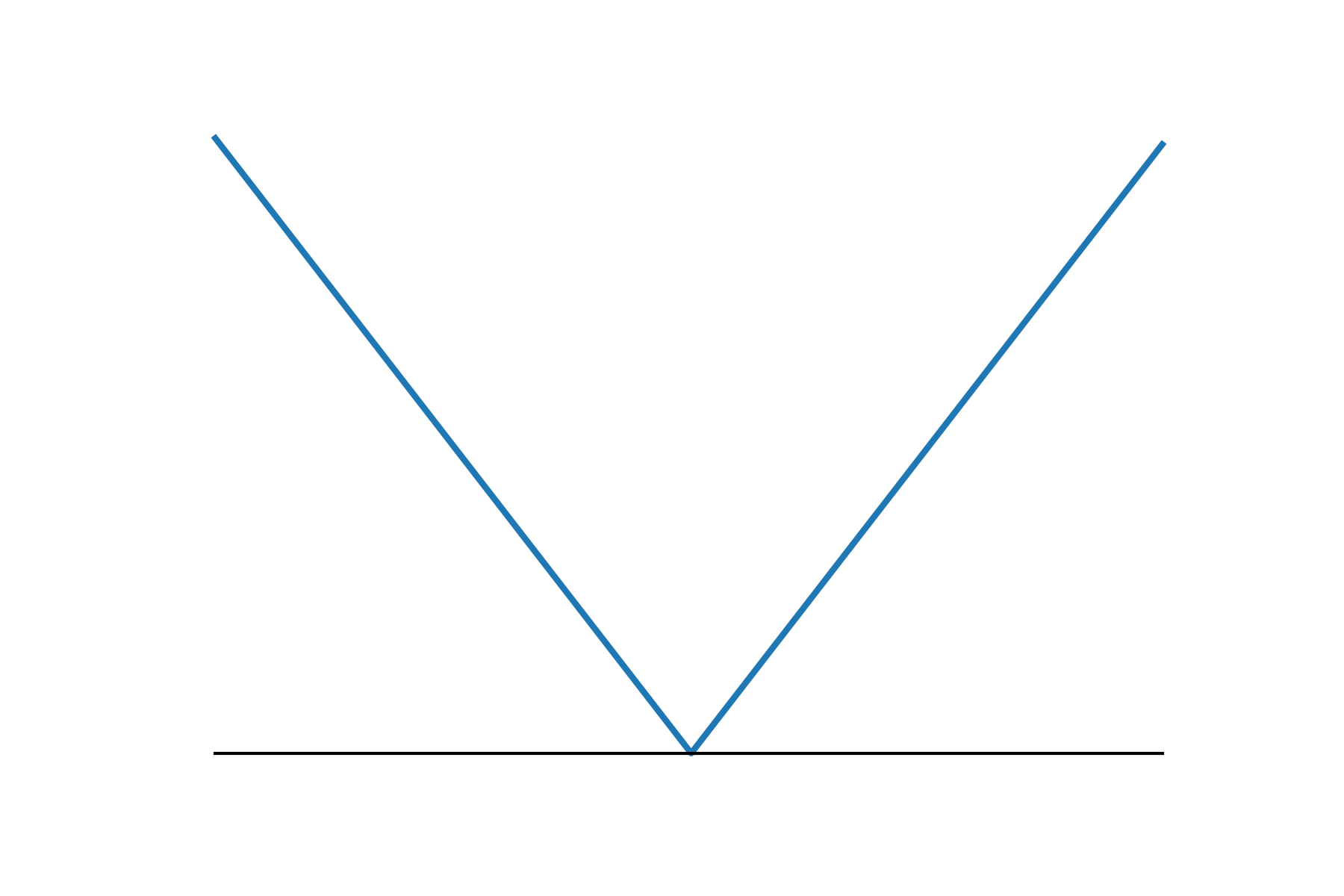
when is nonsmooth:

f

\mathcal{O}(1/\epsilon^2).

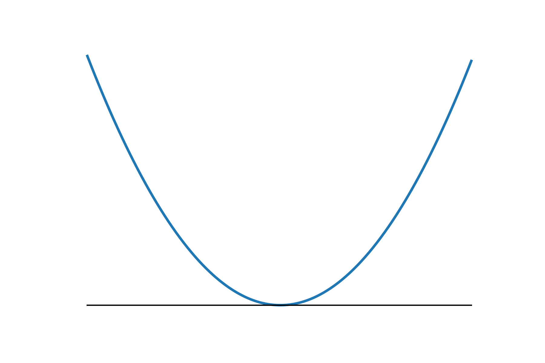
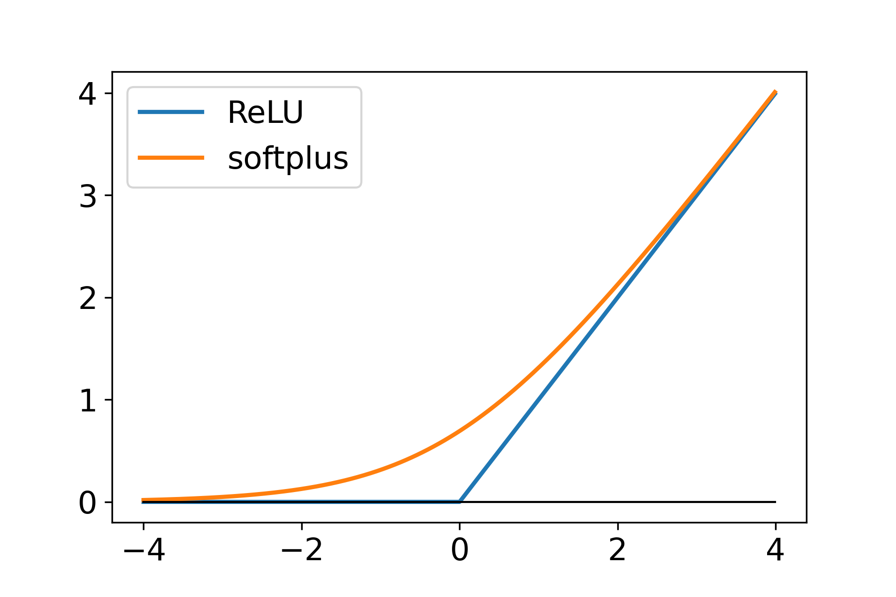
smooth

nonsmooth

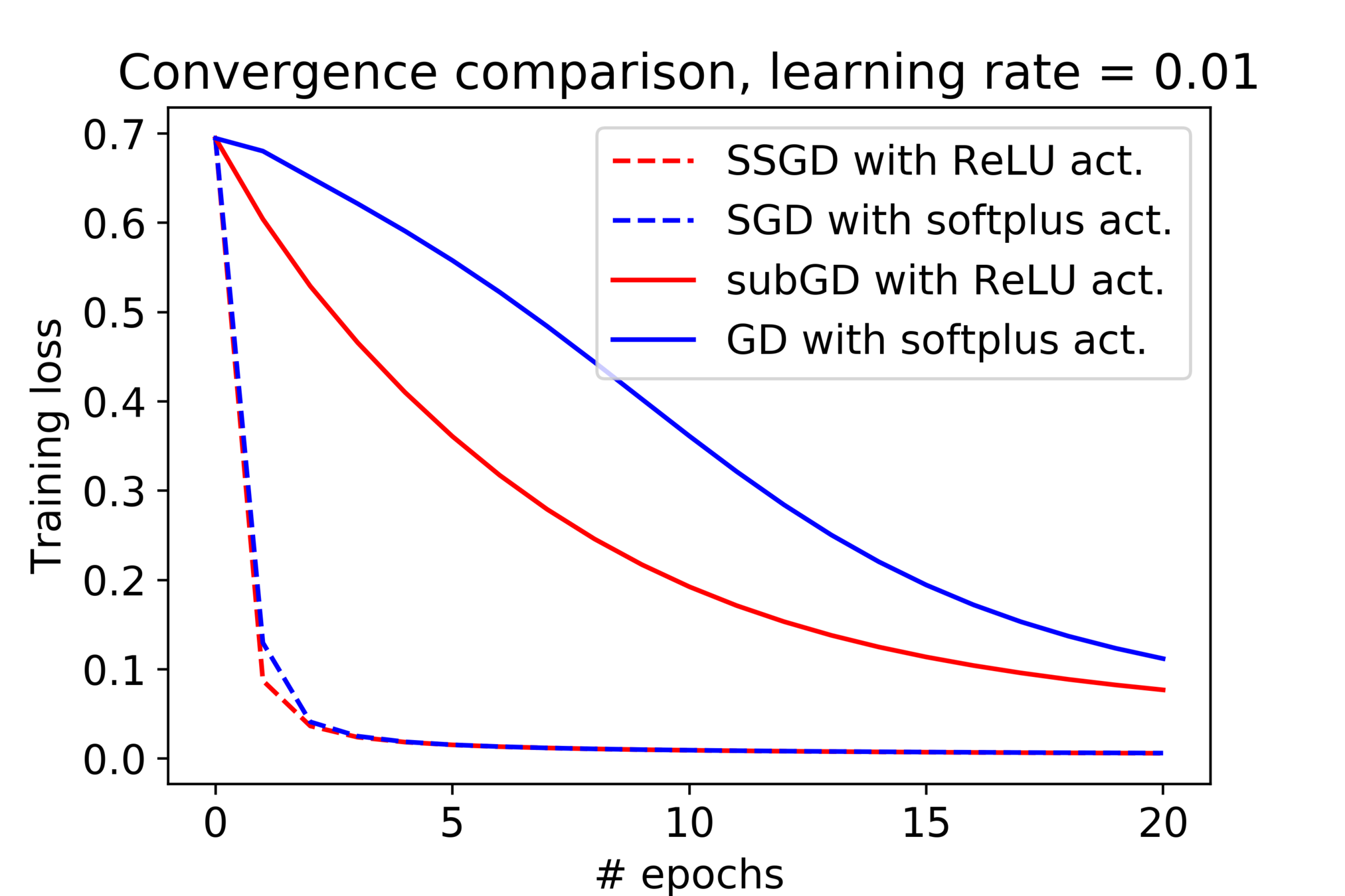
The empirical observation

Some discrepancies between theory and practice:

Nonsmoothness from the model does not slow down our training in practice.

The learning rate schedule can yield optimal iteration complexity but seldom used in practice.

\eta_t \propto 1/\sqrt{t}

Filling the gap

Our assumption:

The objective satisfy certain structure:

\underset{x \in \mathbb{R}^d}{\min}~ f(x) = \frac{1}{n} \sum_{i=1}^n f_i(x) \coloneqq \frac{1}{n} \sum_{i=1}^n \ell(h_i(x)),

where is a nonnegative, , convex, 1-smooth loss function, 's are Lipschitz continuous.

\ell : \mathbb{R} \to \mathbb{R}_{\geq 0}

The interpolation condition: there exist such that

x^*

f(x^*) = 0 .

h_i

We prove

[FFF, ICLR'21]

Convex objective:

Strongly convex objective:

\mathcal{O}(1/\epsilon^2) \to \mathcal{O}(1/\epsilon).

\mathcal{O}(1/\epsilon) \to \mathcal{O}(\log(1/\epsilon)).

Optimal

\inf \ell = 0

The above rates match the rate of SGD for smooth objectives.

Backup slides for CD

GCD for Sparse Optimization

The GS-s rule:

The GS-r rule:

The GS-q rule:

j \in \arg\max_{i \in [d]} \left\{ \min_{s \in \partial g_i(x_i)} | \nabla_i f(x) + s | \right\}

j \in \arg\max_{i \in [d]} \left\{ \left| x_i - \mathrm{prox}_{g_i/L} \left[ x_i - \frac{1}{L} \nabla_i f(x) \right] \right| \right\}

j \in \arg\max_{i \in [d]} \left\{ \min_d\left\{ \nabla_i f(x) d + \frac{Ld^2}{2} + g_i( x_i + d ) - g_i(x_i) \right\} \right\}

\displaystyle \mathrm{prox}_g (x) = \underset{y \in \mathbb{R}^d }{\arg\min}~ \frac{1}{2} \|y - x\|_2^2 + g(y)

Sparsity measure

\delta_i \coloneqq \min\{ -\nabla_i f(x^*) - l_i, u_i + \nabla_i f(x^*) \}

where .

\partial g_i(x^*_i) = [l_i, u_i]

A key property:

| \nabla_i f( x^{(t)} ) - \nabla_i f(x^*) | \leq \delta_i,~x_i^{(t)} = 0,~x_i^* = 0

\Rightarrow \quad x_i^{(t+1)} = 0

The definition of

\delta_i

\|x\|_2 \leq \| x \|_1 \leq \sqrt{d} \| x \|_2

Norm inequality:

Sparsity measure

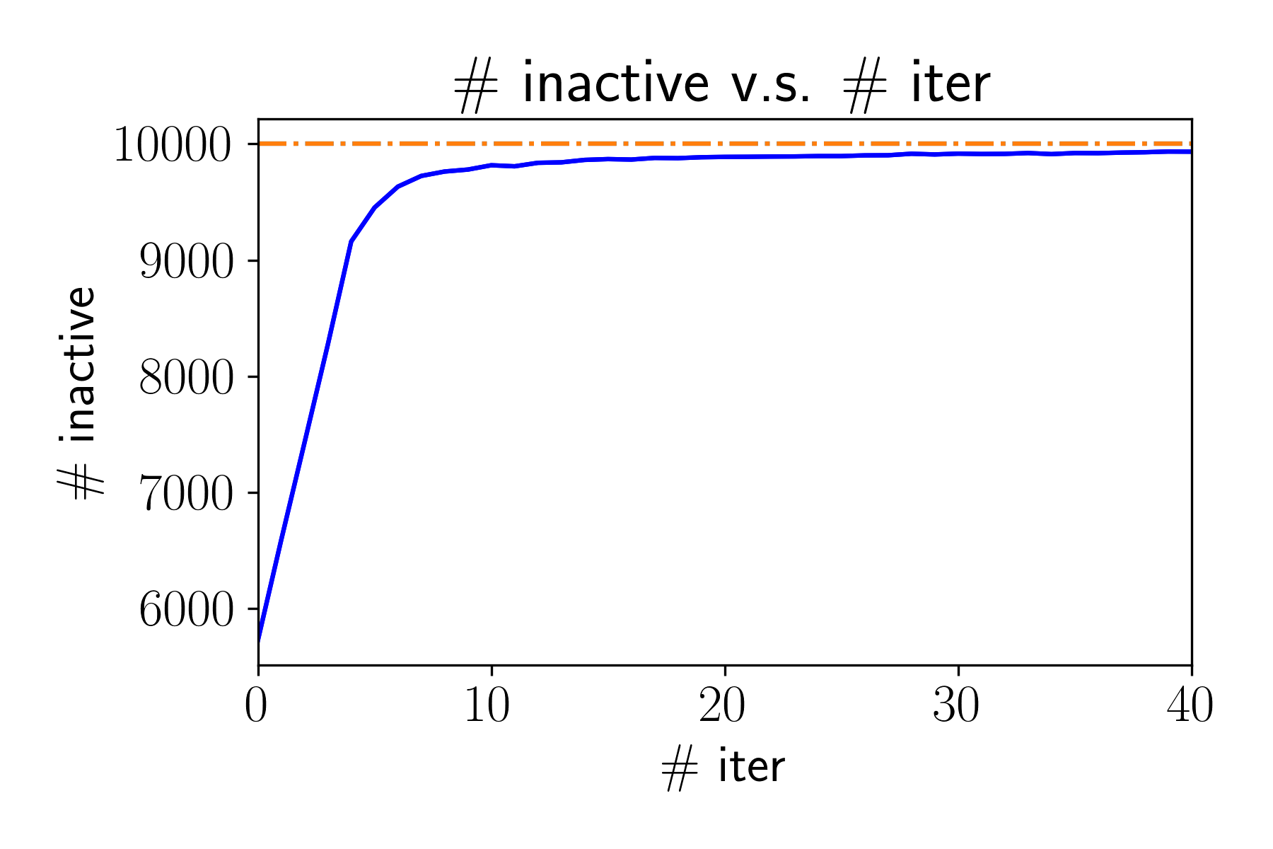
\text{\# inactive} = \sum_{i=1}^d \textbf{1}\left\{ | \nabla_i f(x^{(t)}) - \nabla_i f(x^*) | \leq \delta_i \right\}

F( x^{(t+1)} ) - F^* = (1 - \rho_t)\left( F(x^{(t)}) - F^* \right)

Matrix AMGM inequality

\displaystyle \left\| \frac{1}{n!} \sum_{ \sigma \in \mathrm{Perm}(n) } \prod_{j=1}^n A_{\sigma(j)} \right\| \leq \displaystyle \left\| \frac{1}{n^n} \sum_{ k_1,\ldots,k_n=1 }^n \prod_{j=1}^n A_{k_j} \right\|

for all PSD matrix

A_1, \ldots, A_n \in \mathbb{R}^{d \times d}.

The matrix AMGM inequality conjecture is false [LL20, S20])

Atom identification

\mathcal{F}_\mathcal{A} ( z, \epsilon ) = \{ a \in \mathcal{A} \mid \langle a, z \rangle \geq \sigma_\mathcal{A}(z) - \epsilon \}

\mathcal{F}_\mathcal{A} ( z ) = \{ a \in \mathcal{A} \mid \langle a, z \rangle \geq \sigma_\mathcal{A}(z) \}

where is the support function.

\sigma_{\mathcal{A}}(z) = \sup_{a \in \mathcal{A}} \langle a, z \rangle

x \to x^* \quad {\Rightarrow} \quad \mathrm{supp}(x) \to \mathrm{supp}(x^*)

y \to y^* \quad \Rightarrow \quad \mathcal{F}_{\mathcal{A}}(y, \epsilon) \to \mathcal{F}_{\mathcal{A}}(y^*)

The primal-dual relationship:

\mathrm{supp}(x^*) \subseteq \mathcal{F}_{\mathcal{A}}(y^*)

This allows us to do screening base on dual variable:

Backup slides for OMD

Basics

Bregman divergence

D_\Phi(x, y) \coloneqq \Phi(x) - \Phi(y) - \langle \nabla \Phi(y), x - y \rangle

Properties of mirror map

\Phi : \bar{\mathcal{D}} \to \mathbb{R}^d

is nonempty,

\mathcal{D}

is differentiable on , and

\Phi

\mathcal{D}

, where is the boundary of , i.e.,

\partial \mathcal{D}

\lim_{x \to \partial \mathcal{D}} \| \nabla \Phi(x) \| = + \infty

\mathcal{D}

\partial \mathcal{D} \coloneqq \mathrm{cl} \mathcal{D} ~\backslash~ \mathcal{D}.

\Phi(x) = \frac{1}{2} \| x \|_2^2 ~\Rightarrow~ D_\Phi(x, y) = \frac{1}{2} \| x - y \|_2^2

Examples:

\Phi(x) = \sum_{i=1}^d x_i \log(x_i) ~\Rightarrow~ D_\Phi(x, y) = \sum_{i=1}^d x_i \log(x_i/y_i)

Backup slides for SGD

Basics

	smooth	nonsmooth	smooth+IC	nonsmooth + IC
convex
strong cvx

\mathcal{O}(1/\epsilon)

\mathcal{O}(1/\epsilon^2)

\mathcal{O}(1/\epsilon)

\mathcal{O}(\log(1/\epsilon))

\mathcal{O}(1/\epsilon^2)

\mathcal{O}(1/\epsilon)

Semi-smooth properties

Assume , is -Lipschitz continuous and is nonnegative, convex, 1-smooth, minimum at 0, 1-dimensional function. Then

f(x) \coloneqq \ell( h(x) )

h

L

\ell

\| \partial f(x) \|^2 \leq 2 L^2 f(x)

(the generalized growth condition)

\| \partial f(x) - \partial f(y) \| \leq L^2 \| x - y \| + 2L \sqrt{2\min\{ f(x), f(y) \}}

Extension

High probability error bound

\mathcal{O}( \log(1/\delta)/\epsilon )

Conjecture: variance reduced SGD (SAG, SVRG, SAGA) + generalized Freedman inequality

\to

Simple proof of exponential tail bound

First-order methods for structured optimization

Background and motivation

The literature

Coordinate Optimization

Coordinate Descent

GCD for Sparse Optimization

GCD for Sparse Optimization

From coordinate to atom

Online Mirror Descent

Online Convex Optimization

Mirror Descent (MD) and Dual Averaging (DA)

OMD Algorithm

Stabilized OMD

(Stochastic) Subgradient Method

Smooth v.s. Nonsmooth Minimization

The empirical observation

Filling the gap

Acknowledgment

Thank you! Questions?

Backup slides

Backup slides for CD

GCD for Sparse Optimization

Sparsity measure

Sparsity measure

Matrix AMGM inequality

Atom identification

Backup slides for OMD

Basics

Backup slides for SGD

Basics

Semi-smooth properties

Extension

thesis

thesis

Fang Huang