Data Cleaning & Exploration
using R
Abdullah Fathi

Why Clean and Tidy Data is Necessary for a Successful Analysis
If data cleaning is not part of data analysis, then why is it so important to spend time on it?
What happens if an Analysis is Performed on Raw Data?
Wrong data class prevents calculations to be performed
Missing data prevents
functions to work properly
Outliers corrupt the output and produce bias
The size of the data requires too much computation
Best Table Types in R
What is a Table in R?
data.frame
data.table
data_frame
Introduction to Missing Data Handling
NA
- Missing data is common in raw data
- NA: Not Available or Not Applicable
- There could be various reasons behind NAs
- The amount of missing values matters
- Get information on the missing values from the person providing/creating the dataset
General Categories of Missing Data
MCAR - Missing Completely At Random
- NA's are present due to randomness
- Deleting or replacing the NA's doesn't cause bias
MAR - Missing At Random
- NAs were produced for a random reason
- The reason has nothing to do with the observation
- Standard imputation methods can solve the issue
MNAR - Missing Not At Random
- NA's are present for a reason
- Some observation cannot be captured properly
- The NA's cause corruption in analysis
Simple Methods for Missing Data Handling
Deleting
Amount of NA's is < 5% and they are MCAR
Hot Deck Imputation
- Replacing NA's with another observation (eg: LOCF)
- Can cause bias !
Imputation with mean
Replacing NA's with the mean, results in less bias
Interpolation
Replacement is identified via a pre-defined algorithm
Simple Methods (Deleting, Hot Deck Imputation, Mean Imputation, Interpolation)
- They do not account for uncertainty
Multiple Imputation Method
- Calculate m number of values as replacement
- A copy of the dataset for each set of replacement is generated
- Analysis is performed on each copy
- Average, variance and confidence intervals are taken from the pool
- They work on MAR and MNAR datasets too
- MICE - Multiple Imputation by Chained Equation
Simple Methods
(Level of Complexity)
Use a function with a built-in NA handling feature
Use a basic function dedicated to NA handling
Use an advanced imputation tool
Using ML algorithms for missing data handling
- Complex yet effective method
- Library/Package 'MICE'
- various multiple imputation method
Outliers
An outlier is an observation which deviates from the other observations as to arouse suspicions that it was generated by a different mechanism - Hawkins
An Outlier is an observation that is significantly different from the generating mechanism or a statistical process - Statistician
Even a couple of outliers can completely change the result
What to do with outliers?
Leave them as they are
Delete them
Exchange them with another value
Deleting and Exchanging Outlier
Deleting and exchanging methods have their drawbacks with small samples
Assumption: The data point is faulty
An outlier totally out of scale might be a wrong measurement
- Not likely when measurements are automated
- Human mistakes are more likely to occur
- Example: Plausibility checks in clinical research
Outliers can be valid measurements and they might reveal hidden potentials
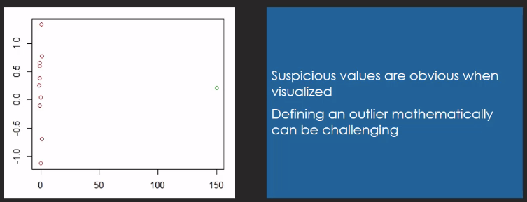
Scatterplot with Outlier
Tidyverse for efficient data cleaning
Tidyverse
- A collection of packages that work together
- The whole package can be pulled with the command install.packages("tidyverse")
- > 70 libraries/packages
- Conflicts can occur
- Recommendation: Install only the packages you need (+dependencies)
What is the Tidyverse?
- A collection of packages written and maintained by the RStudio Team
- Major contributions by Hadley Wickham
eg: "ggplot2", "dplyr"
- Major contributions by Hadley Wickham
- Libraries/packages in the collection work together seamlessly in order to achieve clean and tidy data
- Basic principles of the Tidyverse:
- Pipe operator %>%
- Functional programming
- Memory efficiency
Core Packages in Tidyverse
- library(tidyverse)
- ggplot2
- dplyr
- tidyr
- readr
- purr
- tibble
- stringr
- forcats
- The rest of the Tidyverse packages need to be activated individually (eg: "lubridate", "hms")
ggplot2
- Library for complex and high quality data visualizations
- Popular and frequently used in data science
- Specific syntax:
- Similar to the pipe operator (%>%)
- Sub-language
dplyr
- Library for manipulating data.frame and similar structures
- Popular and frequently used in data science
- Interact with the "tibble" library
- Specialities:
- Joining, sorting, querying and rearranging data.frames
- Getting various summary statistics
- Addition of new columns
- An alternative to R base
tidyr
- Library for data cleaning, tidying
- Functions for:
- data pre-processing
- cleaning
- conversion of long and wide formats
- splitting and merging columns
readr
- Library for data importing
- Functionalities are implemented in the RStudio interface
- Warnings for data irregularities
purr
- Library for functional programming
- Write your own R functions
- For advanced users and people coming from other languages
tibble
- Library of the "tibble" object
- Tibble replaces "data_frame" in dplyr
- An alternative for "data.frame" and "data.table"
- Tibble object eliminate some disadvantages of other df objects
- Uncontrolled recycling
- Keeping character columns
- Providing better information on classes
stringr
- Library for string manipulations
- Upper and lowercase conversion
- Splitting or merging texts
- Finding specific letter combinations
- Improved functionalities compared to standard "gsub" operations
forcats
- Library for factor manipulations
- Factor: A categorical variable
- Counting observations of a category
- Fusing categories
- Relabeling categories
Does tidyverse offer a solution to all data science tasks and challenge?
Tidyverse Main focus on
Data Pre-Processing
Importing Data
Data Cleaning
Data Visualization
Custom Functions
Pipe Operator %>%
- The pipe operator %>%
- Library "magrittr" - dependency for most Tidyverse packages
- The pipe changes the R syntax - sub-language
- Makes the syntax more intuitive
- Makes coding of advanced objects easier
- Good documentation
- Packages by the RStudio Team prefer that coding style
Limitations of the pipe operator
- Number of pipe operations in an object should not be more than 10
- Easier troubleshooting
- Single Input
- Single Output
- Multiple outputs: apply family of functions
Further Operators of Library "magrittr"
%$%
Alternative to attach()
%<>%
Alternative to assign()
%T>%
Inserting an intermediary step
Tibble as Alternative to the "data.frame"
- Class "data.frame" -> commonly used in R
- Improved class: "tibble" -> Tidyverse
- "tibble" = "data_frame"
- Change in function:
tbl_df-> tibble() - Class of "tibble" is still called "tbl_df" in R!
Recycling: "data.frame" vs "tibble"
A "data.frame" and a new column can be of different length -> recycling
A "tibble" and the newly provided data have to be of equal length -> no recycling
Exception: single value
Summary of tibble
- Never recycles except for a length of one
- Never changes column names
- Never uses row names
- Never changes classes while importing data
- Main Functions:
- tibble() - Creates a "tibble" from scratch
- tribble() - Creates a "tibble" from scratch by rows
- as.tibble() - Converts a data frame into a "tibble"
- add_row() - Adds extra rows to the "tibble"
- add_column() - Adds extra columns to the "tibble"
Tidy Data as the Underlying Principle of the Tidyverse
Raw Data
Tidy Data
Different data types and classes require specific cleaning methods
Library(tidyr)
- The core package of the Tidyverse
- Organizing data into a tidy "tibble"
- Focus lays on the whole table format
- Classes of tables in R:
- data.frame
- data.table
- data_fram(tibble)
Three rules of Tidy Data
Each variable has its own column
Each observation has its own row
Each observational unit forms one table
Converting From Wide to Long Format
Converting From Long to Wide Format
String Manipulations
Character/String: Text data or data R considers text ("string")
Column Separation
String Manipulations in R
- Computer settings and locale might affect the encoding of string values
- Some functions are sensitive to encoding issues e.g. gsub()
- Text analysis is a hot topic of today's data science (eg: web scraping, sentiment analysis, data mining)
- R Base: gsub() and its sub-language "regex"
- Library "stringr": a collection of functions for the most common string handling problems
Summary of "stringr"
- str_c(): combines strings or string vectors
- str_count(): counts the occurrences of a character combination in a string
- str_replace(): finds and replaces a character combination in a string (first occurrence only)
- str_replace_all(): finds and replaces all occurrences of a character combination in a string
- str_to_upper(): uppercase conversion
- str_to_lower(): lowercase conversion
- str_length(): returns the number of characters in a string
- str_pad(): pads a string to a given length
- "left": "XXXXXXapple"
- "right": "appleXXXXXX"
- "both": "XXXappleXXX"
Exploratory Data Analysis
Query systems in R
- Selecting a subset of data that fits specific criteria provided by the analyst
- Combination of criteria is possible
- Querying different classes of tables
- data.frame
- data.table
- tibble
- Querying functions of the library "dplyr"
Filtering and Queries
- Last steps of the cleaning process
- Querying/filtering/sub-setting: pulling specific parts of the dataset based on certain criteria
- Reordering data based on one or more criteria
- SQL like structures integrated into R
- Table types:
- data.frame - basic toolset
- data.table - intuitive syntax, fast computation
- tibble - queried similarly to a data.frame
- Different table types (data.frame, data.table, tibble) are queried similarly
- dataset[rows, columns]
- Results might differ depending on the table type the query is performed on
- DFdata not equal to DTdata[3]
- Tibbles and data.frames are queried similarly
- Data.table queries require less coding and are more efficient on large datasets
Single Table Verbs
Library "dplyr"
Library(dplyr)
- A popular library for data management in R
- Tools for SQL integration and database normalization
- Intuitive structure: functions are named as verbs
- eg: arrange(), filter()
- Efficient data storage
- Fast processing
Library(dplyr)
- Cover all required steps of data manipulation and data management
- arrange(): to reorder rows
- filter(): to pick observations
- slice(): to pick observations by Order ID
- select(): to pick variables
- mutate(): to add new variables
- summarize(): to collapse variables
- sample_n(): to select random rows from a table
- Can be used on tidy, well structured datasets
Merge with dplyr()
We may have many sources of input data, and at some point, we need to combine them. A join with dplyr adds variables to the right of the original dataset. The beauty is dplyr is that it handles four types of joins similar to SQL
-
left_join()
-
right_join()
-
inner_join()
-
full_join()
install.packages("dplyr")1. left_join()
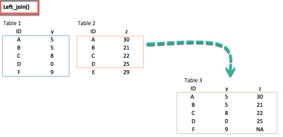
left_join(df_primary, df_secondary, by ='ID')2. right_join()
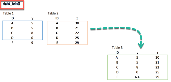
right_join(df_primary, df_secondary, by = 'ID')Multiple keys pairs
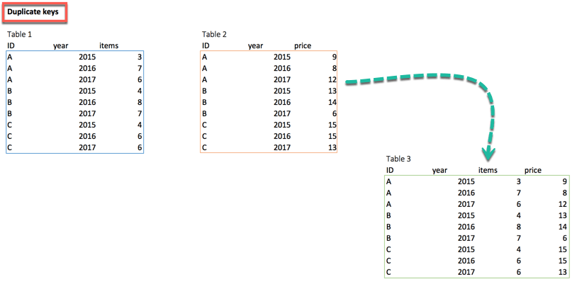
left_join(df_primary, df_secondary, by = c('ID', 'year'))we can have multiple keys in our dataset. Consider the following dataset where we have years or a list of products bought by the customer.
3. inner_join()
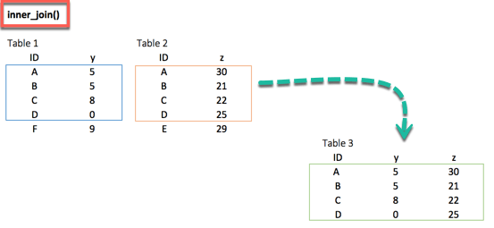
inner_join(df_primary, df_secondary, by ='ID')When we are 100% sure that the two datasets won't match, we can consider to return only rows existing in both dataset
4. full_join()
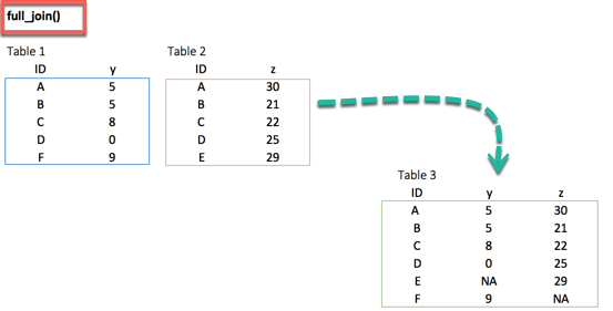
full_join(df_primary, df_secondary, by = 'ID')full_join() function keeps all observations and replace missing values with NA.
Basic function
Subsetting
The function summarise() is compatible with subsetting.
Sum
Another useful function to aggregate the variable is sum().
Standard deviation
Spread in the data is computed with the standard deviation or sd() in R
Minimum and maximum
Access the minimum and the maximum of a vector with the function min() and max().
Count
Count observations by group is always a good idea. With R, we can aggregate the the number of occurence with n()
First and last
Select the first, last or nth position of a group
nth observation
The function nth() is complementary to first() and last(). We can access the nth observation within a group with the index to return
Distinct number of observation
The function n() returns the number of observations in a current group. A closed function to n() is n_distinct(), which count the number of unique values
Multiple groups
A summary statistic can be realized among multiple groups
Filter
Before we intend to do an operation, we can filter the dataset
Ungroup
We need to remove the grouping before we want to change the level of the computation
Summarise()
The syntax of summarise() is basic and consistent with the other verbs included in the dplyr library
summarise(df, variable_name=condition)
# arguments:
# - `df`: Dataset used to construct the summary statistics
# - `variable_name=condition`: Formula to create the new variable
Group_by
vs
no group_by
group_by works perfectly with all the other verbs (i.e. mutate(), filter(), arrange(), ...)
Combining group_by(), summarise() and ggplot() together
- Step 1: Select data frame
- Step 2: Group data
- Step 3: Summarize the data
- Step 4: Plot the summary statistics
Function in summarise()
|
Basic |
mean() |
Average of vector x |
|
|
median() |
Median of vector x |
|
|
sum() |
Sum of vector x |
|
variation |
sd() |
standard deviation of vector x |
|
|
IQR() |
Interquartile of vector x |
|
Range |
min() |
Minimum of vector x |
|
|
max() |
Maximum of vector x |
|
|
quantile() |
Quantile of vector x |
|
Position |
first() |
Use with group_by() First observation of the group |
|
|
last() |
Use with group_by(). Last observation of the group |
|
|
nth() |
Use with group_by(). nth observation of the group |
|
Count |
n() |
Use with group_by(). Count the number of rows |
|
|
n_distinct() |
Use with group_by(). Count the number of distinct observations |
Objective
Function
Description
Visualisation
Scatter plot with ggplot2
Graphs are an incredible tool to simplify complex analysis
Graphs are the third part of the process of data analysis. The first part is about data extraction, the second part deals with cleaning and manipulating the data. At last, we need to visualize our results graphically.
ggplot2 package
ggplot2 is very flexible, incorporates many themes and plot specification at a high level of abstraction. With ggplot2, we can't plot 3-dimensional graphics and create interactive graphics
The basic syntax of ggplot2 is:
ggplot(data, mapping=aes()) +
geometric object
# arguments:
# data: Dataset used to plot the graph
# mapping: Control the x and y-axis
# geometric object: The type of plot you want to show. The most common object are:
# - Point: `geom_point()`
# - Bar: `geom_bar()`
# - Line: `geom_line()`
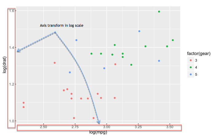
# - Histogram: `geom_histogram()`Change axis
One solution to make our data less sensitive to outliers is to rescale them
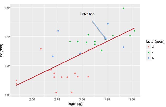
Scatter plot with fitted values
We can add another level of information to the graph. We can plot the fitted value of a linear regression.
Add information to the graph
Graphs need to be informative and good labels. We can add labels with labs()function
lab(title = "Hello Fathi")
# argument:
# - title: Control the title. It is possible to change or add title with:
# - subtitle: Add subtitle below title
# - caption: Add caption below the graph
# - x: rename x-axis
# - y: rename y-axis
# Example:lab(title = "Hello Fathi", subtitle = "My first plot")
Theme
The library ggplot2 includes eights themes:
- theme_bw()
- theme_light()
- theme_classis()
- theme_linedraw()
- theme_dark()
- theme_minimal()
- theme_gray()
- theme_void()
Save Plots
ggsave("my_fantastic_plot.png")Store graph right after we plot it
How to make Boxplot in R
Box plot helps to visualize the distribution of the data by quartile and detect the presence of outliers
Bar Chart & Histogram
Bar chart is a great way to display categorical variables in the x-axis. This type of graph denotes two aspects in the y-axis.
- The first one counts the number of occurrence between groups.
- The second one shows a summary statistic (min, max, average, and so on) of a variable in the y-axis
How to create Bar Chart
ggplot(data, mapping = aes()) +
geometric object

# arguments:
# data: dataset used to plot the graph
# mapping: Control the x and y-axis
# geometric object: The type of plot you want to show. The most common objects are:

# - Point: `geom_point()`
# - Bar: `geom_bar()`
# - Line: `geom_line()`
# - Histogram: `geom_histogram()`
Customize the graph
# - `stat`: Control the type of formatting. By default, `bin` to plot a count in the y-axis. For continuous value, pass `stat = "identity"`
# - `alpha`: Control density of the color
# - `fill`: Change the color of the bar
# - `size`: Control the size the bar
Four arguments can be passed to customize the graph
Histogram
Represent the group of variables with values in the y-axis
R Interactive Map (leaflet)
Leaflet is one of the most popular open-source JavaScript libraries for interactive maps
Leaflet Package
install.packages("leaflet")
# to install the development version from Github, run
# devtools::install_github("rstudio/leaflet")
Correlation
Pearson Correlation
- Usually used as a primary check for the relationship between two variables
- The coefficient of correlation, is a measure of the strength of the linear relationship between two variables.
- The correlation ranges between -1 and 1
- A value of near or equal to 0 implies little or no linear relationship between variables
- The closer comes to 1 or -1, the stronger the relationship
Spearman Correlation
- A rank correlation sorts the observation by rank and computes the level of similarity between the rank
- Has the advantage of being robust to outliers and is not linked to the distribution of the data
- Rank correlation is suitable for the ordinal data
- Spearman's rank correlation is always between -1 and 1 with a value close to the extremity indicates strong relationship
There are no secrets to success. It is the result of preparation, hard work, and learning from failure. - Colin Powell
THANK YOU
R - Data Cleaning & Exploration
By Abdullah Fathi


