R Programming Language
Abdullah Fathi

Introduction to R

History
- R is a programming language
- An implementation over S language
- Designed by Ross Ihaka and Robert Gentleman at the University of Auckland in 1993
- Stable released on 31 October 2014 (3 years ago), by R Development Core Team Under GNU General Public License

What is R?
- Open source
- Cross Platform compatible
- Numerical and graphical analysis
- Large user community
- 9000+ extensions
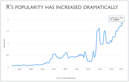
Why Learn R?
- One of the fastest growing programming language
-
R is widely used (statisticians, scientists, social scientists) and has the widest statistical functionality of any software
-
As a scripting language, R is very powerful, flexible, and easy to use
- Quality Graph
How to install R / R Studio ?
- Go to https://www.rstudio.com/products/rstudio/download/
- In ‘Installers for Supported Platforms’ section, choose and click the R Studio installer based on your operating system. The download should begin as soon as you click.
- Click Next..Next..Finish.
- Download Complete.
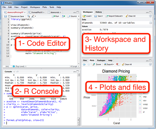

RStudio Interface
- R Console: This area shows the output of code you run. Also, you can directly write codes in console. Code entered directly in R console cannot be traced later. This is where R script comes to use.
- Code Editor: As the name suggest, here you get space to write codes. To run those codes, simply select the line(s) of code and press Ctrl + Enter. Alternatively, you can click on little ‘Run’ button location at top right corner of R Script.
- Workspace & History: This space displays the set of external elements added. This includes data set, variables, vectors, functions etc. To check if data has been loaded properly in R, always look at this area.
- Plot & Files: This space display the graphs created during exploratory data analysis. Not just graphs, you could select packages, seek help with embedded R’s official documentation.
Install R Packages
install.packages("package name")
Install R Packages
Programmatically
if (!require(dplyr)) {
  install.packages("dplyr")
  library(dplyr)
}
R Data Types & Operator
Basic Data Type
-
Character: Value inside "" or '' are text(string).
-
Numeric (Real Numbers): 4.5 is a decimal value
-
Integer (Whole Numbers): 4 is a natural value
-
Logical (TRUE/FALSE)
Check the type of a variable with the class function
# Declare variables of different types
# Numeric
x <- 28
class(x)
Variables
-
A variable can store a number, an object, a statistical result, vector, dataset, a model prediction basically anything R outputs
-
We can use that variable later simply by calling the name of the variable
-
To declare a variable, we need to assign a variable name. The name should not have space. We can use _ to connect to words
Assign Operator
Create variable using <- or = sign
| OPERATOR | DESCRIPTION | EXAMPLE |
|---|---|---|
| x + y | y added to x | 2 + 3 = 5 |
| x – y | y subtracted from x | 8 – 2 = 6 |
| x * y | x multiplied by y | 3 * 2 = 6 |
| x / y | x divided by y | 10 / 5 = 2 |
| x ^ y (or x ** y) | x raised to the power y | 2 ^ 5 = 32 |
| x %% y | remainder of x divided by y (x mod y) | 7 %% 3 = 1 |
| x %/% y | x divided by y but rounded down (integer divide) | 7 %/% 3 = 2 |
Arithmetic Operators
Logical Operators
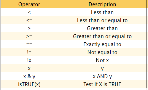
We can add many conditional statements as we like but we need to include them in a parenthesis
# Create a vector from 1 to 10
logical_vector <- c(1:10)
logical_vector>5

# Print value strictly above 5
logical_vector[(logical_vector>5)]
Data Types
-
Vector
-
Matrices
-
Factor
-
Data Frame
-
List
1. Vector
- A vector contains object of same class. But, you can mix objects of different classes too. When objects of different classes are mixed in a list, coercion occurs.This effect causes the objects of different types to ‘convert’ into one class
- We can do arithmetic calculations on vectors.
The simplest way to build a vector in R, is to use the
c command
# Numerical
vec_num <- c(1, 10, 49)
vec_num

# Character
vec_chr <- c("a", "b", "c")
vec_chr

# Boolean
vec_bool <-  c(TRUE, FALSE, TRUE)
vec_bool
Slice a vector
# Slice the first five rows of the vector
slice_vector <- c(1,2,3,4,5,6,7,8,9,10)
slice_vector[1:5]
Shortest way to create a range of value is to use the
':' between two numbers
# Faster way to create adjacent values
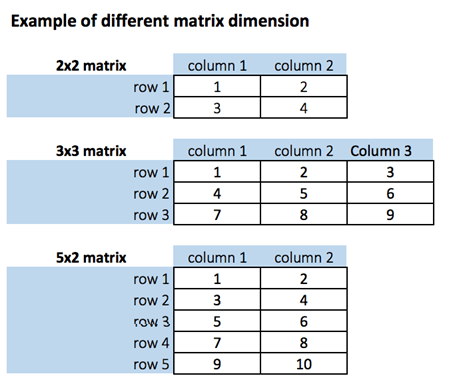
c(1:10)2. Matrices
A matrix is a 2-dimensional array that has m number of rows and n number of columns. In other words, matrix is a combination of two or more vectors with the same data type.
matrix(data, nrow, ncol, byrow = FALSE)
# Arguments:
# - data: The collection of elements that R will arrange into the rows and columns of the matrix
# - nrow: Number of rows
# - ncol: Number of columns
# - byrow: The rows are filled from the left to the right. We use `byrow = FALSE` (default values), if we want the # matrix to be filled by the columns i.e. the values are filled top to bottom. - We can create a matrix with the function matrix(). This function takes three arguments:
- Get Matrix Dimension
# Print dimension of the matrix with dim()
dim(matrix_a)
# concatenate c(1:5) to the matrix_a
matrix_a1 <- cbind(matrix_a, c(1:5))
# Check the dimension
dim(matrix_a1)- add a column to a matrix with the cbind() command. cbind() means column binding
- Add row to a matrix with the rbind() command. rbind() appends rows.
matrix_c <-matrix(1:12, byrow = FALSE, ncol = 3)
# Create a vector of 3 columns
add_row <- c(1:3)
# Append to the matrix
matrix_c <- rbind(matrix_c, add_row)
# Check the dimension
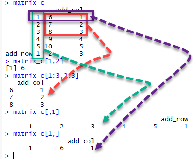
dim(matrix_c)Slice a Matrix
We can select elements one or many elements from a matrix by using the square brackets [ ].
- matrix_c[1,2] selects the element at the first row and second column.
- matrix_c[1:3,2:3] results in a matrix with the data on the rows 1, 2, 3 and columns 2, 3,
- matrix_c[,1] selects all elements of the first column.
- matrix_c[1,] selects all elements of the first row.
3. Factor
Type of variable that is essentially used to refer to qualitative/categorical variable
In a dataset, we can distinguish two types of variables: categorical and continuous.
Categorical Variables
R stores categorical variables into a factor. Characters are not supported in machine learning algorithm, and the only way is to convert a string to an integer.
factor(x = character(), levels, labels = levels, ordered = is.ordered(x))
# Arguments:
# - x: A vector of data. Need to be a string or integer, not decimal.
# - Levels: A vector of possible values taken by x. This argument is optional. The default value is the unique list of # items of the vector x.
# - Labels: Add a label to the x data. For example, 1 can take the label `male` while 0, the label `female`.
# - ordered: Determine if the levels should be ordered. - It is important to transform a string into factor when we perform Machine Learning task.
- A categorical variable can be divided into nominal categorical variable and ordinal categorical variable.
A categorical variable has several values but the order does not matter. For instance, male or female categorical variable do not have ordering.
Nominal categorical variable
Ordinal categorical variables do have a natural ordering. We can specify the order, from the lowest to the highest with order = TRUE and highest to lowest with order = FALSE.
Ordinal categorical variable
Continuous class variables are the default value in R. They are stored as numeric or integer.
Continuous variables
4. Data Frame
This is the most commonly used member of data types family. It is used to store tabular data. It is different from matrix. In a matrix, every element must have same class. But, in a data frame, you can put list of vectors containing different classes. This means, every column of a data frame acts like a list.
How to create a data frame
We can create a data frame by passing the variable a,b,c,d into the data.frame() function. We can name the columns with name() and simply specify the name of the variables
data.frame(df, stringsAsFactors = TRUE)
# arguments:
# -df: It can be a matrix to convert as a data frame or a collection of variables to join
# -stringsAsFactors: Convert string to factor by default
Change the column name with the function names()
# Name the data frame
names(df) <- c('ID', 'items', 'store', 'price')
Slice Data Frame
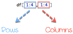
A data frame is composed of rows and columns, df[A, B]. A represents the rows and B the columns. We can slice either by specifying the rows and/or columns.
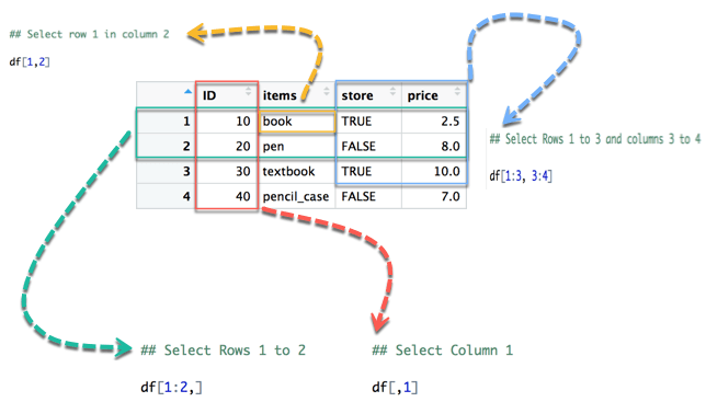
In below diagram we display how to access different selection of the data frame:
- The yellow arrow selects the row 1 in column 2
- The green arrow selects the rows 1 to 2
- The red arrow selects the column 1
- The blue arrow selects the rows 1 to 3 and columns 3 to 4
Append a Column to Data Frame
You can also append a column to a Data Frame. You need to use the symbol $ to append a new variable.
# Create a new vector
quantity <- c(10, 35, 40, 5)

# Add `quantity` to the `df` data frame
df$quantity <- quantity
df
Select a column of a data frame
Sometimes, we need to store a column of a data frame for future use or perform operation on a column. We can use the $ sign to select the column from a data frame
# Select the column ID
df$ID
Subset a data frame
Sometimes, we need to store a column of a data frame for future use or perform operation on a column. We can use the $ sign to select the column from a data frame
subset(x, condition)
# arguments:
# - x: data frame used to perform the subset
# - condition: define the conditional statement
We can get a quick look at the bottom of the data frame with tail() function. By analogy, head() displays the top of the data frame
head(df)
tail(df)
5. List
A list is a great tool to store many kinds of object in the order expected. We can include matrices, vectors data frames or lists.
list(element_1, ...)
# arguments:
# -element_1: store any type of R object
# -...: pass as many objects as specifying. each object needs to be separated by a comma
Select elements from list
- After we built our list, we can access it quite easily. We need to use the [[index]] to select an element in a list.
- The value inside the double square bracket represents the position of the item in a list we want to extract
# Print second element of the list
my_list[[2]]
Sorting
Sort a vector of continuous variable or factor variable. Arranging the data can be of ascending or descending order
Order
order() returns the indices of the vector in sorted order
order(x):
# Argument:
# -x: A vector containing continuous or factor variable
Sort
the result of sort() is a vector consisting of elements of the original (unsorted) vector
sort(x, decreasing = FALSE, na.last = TRUE):
# Argument:
# -x: A vector containing continuous or factor variable
# -decreasing: Control for the order of the sort method. By default, decreasing is set to `FALSE`.
# -na.last: Indicates whether the `NA` 's value should be put last or not
R dplyr
Introduction to Data Analysis
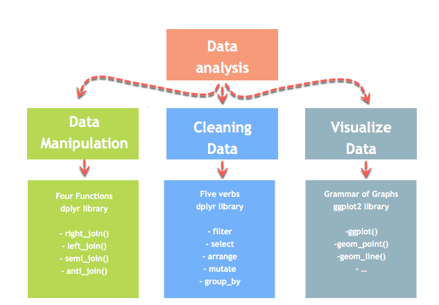
Data analysis can be divided into three parts
- Extraction: First, we need to collect the data from many sources and combine them.
- Transform: This step involves the data manipulation. Once we have consolidated all the sources of data, we can begin to clean the data.
- Visualize: The last move is to visualize our data to check irregularity.
Merge with dplyr()
We may have many sources of input data, and at some point, we need to combine them. A join with dplyr adds variables to the right of the original dataset. The beauty is dplyr is that it handles four types of joins similar to SQL
-
left_join()
-
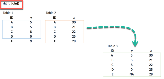
right_join()
-
inner_join()
-
full_join()
install.packages("dplyr")1. left_join()
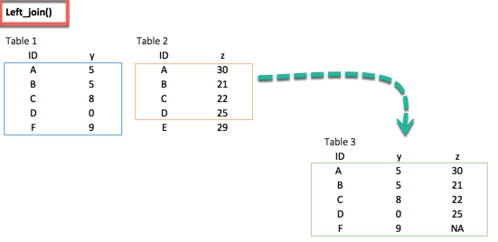
left_join(df_primary, df_secondary, by ='ID')2. right_join()
right_join(df_primary, df_secondary, by = 'ID')3. inner_join()
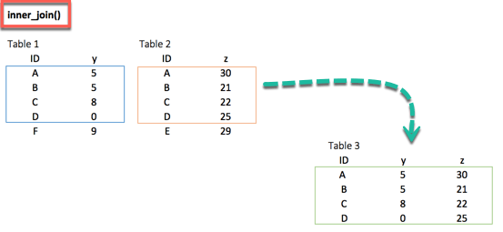
inner_join(df_primary, df_secondary, by ='ID')When we are 100% sure that the two datasets won't match, we can consider to return only rows existing in both dataset
4. full_join()
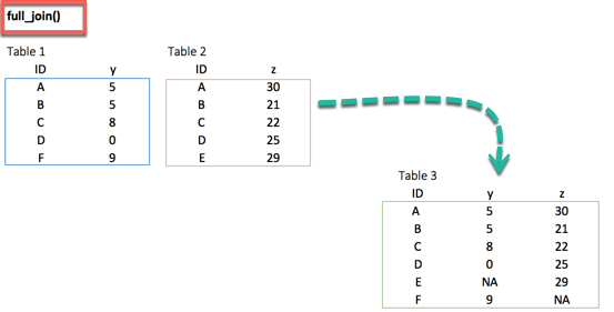
full_join(df_primary, df_secondary, by = 'ID')full_join() function keeps all observations and replace missing values with NA.
Multiple keys pairs
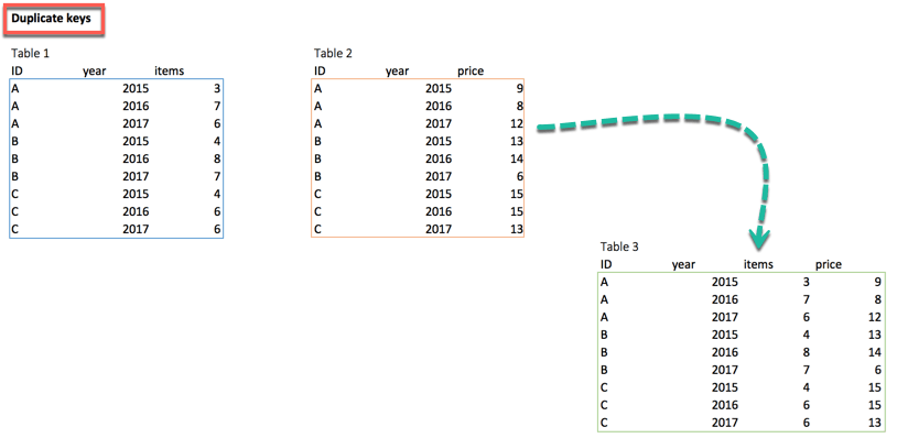
left_join(df_primary, df_secondary, by = c('ID', 'year'))we can have multiple keys in our dataset. Consider the following dataset where we have years or a list of products bought by the customer.
Sort Data Frame
arrange(.data, ...)
# Argument:
# - .data: data frame variable.
# - ...: Comma separated list of unquoted variable names.
The dplyr function arrange() can be used to reorder (sort) rows by one or more variables.
Data Cleaning Functions
4 functions to tidy our data using tidyr
-
gather(): Transform the data from wide to long
-
spread(): Transform the data from long to wide
-
separate(): Split one variable into two
-
unite(): Unit two variables into one
install.packages("tidyr")1. gather()
The objectives of the gather() function is to transform the data from wide to long
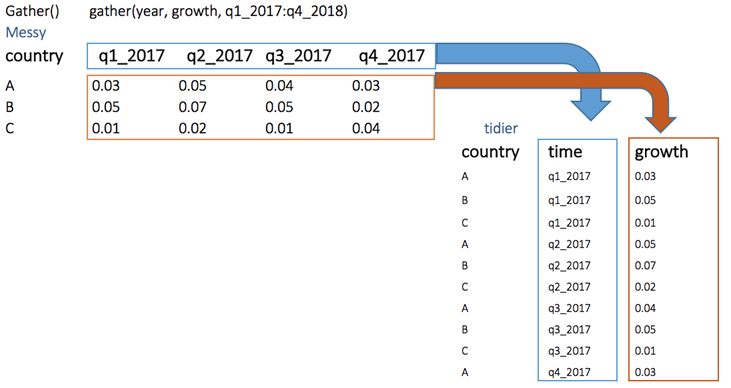
gather(Messy, quarter, growth, q1_2017:q4_2017)2. spread()
The spread() function does the opposite of gather.
spread(data, key, value)

# arguments:
# data: The data frame used to reshape the dataset
# key: Column to reshape long to wide
# value: Rows used to fill the new column
3. separate()
The separate() function splits a column into two according to a separator. This function is helpful in some situations where the variable is a date.
separate(data, col, into, sep= "", remove = TRUE)
# arguments:
# -data: The data frame used to reshape the dataset
# -col: The column to split
# -into: The name of the new variables
# -sep: Indicates the symbol used that separates the variable, i.e.:  "-", "_", "&"
# -remove: Remove the old column. By default sets to TRUE.
4. unite()
The unite() function concanates two columns into one.
unite(data, col, conc ,sep= "", remove = TRUE)
# arguments:
# -data: The data frame used to reshape the dataset
# -col: Name of the new column
# -conc: Name of the columns to concatenate
# -sep: Indicates the symbol used that unites the variable, i.e:  "-", "_", "&"
# -remove: Remove the old columns. By default, sets to TRUE
Merge Data Frames
Normally, we have data from multiple sources. To perform an analysis, we need to merge two dataframes together with one or more common key variables
Full Match
A full match returns values that have a counterpart in the destination table. The values that are not match won't be return in the new data frame. The partial match, however, return the missing values as NA.
We will see a simple inner join. The inner join keyword selects records that have matching values in both tables. To join two datasets, we can use merge() function
merge(x, y, by.x = x, by.y = y)
# Arguments:
# -x: The origin data frame
# -y: The data frame to merge
# -by.x: The column used for merging in x data frame. Column x to merge on
# -by.y: The column used for merging in y data frame. Column y to merge on
Partial Match
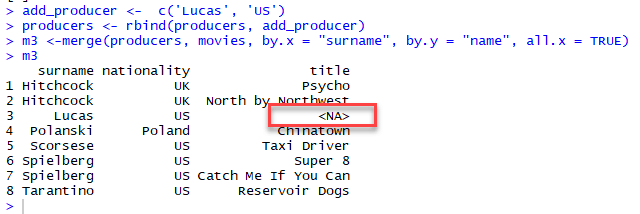
It is not surprising that two dataframes do not have the same common key variables. In the full matching, the dataframe returns only rows found in both x and y data frame.
With partial merging, it is possible to keep the rows with no matching rows in the other data frame. These rows will have NA in those columns that are usually filled with values from y. We can do that by setting all.x= TRUE
Understand the different types of merge
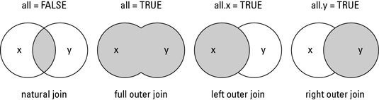
The merge() function allows four ways of combining data:
-
Natural join: To keep only rows that match from the data frames, specify the argument all=FALSE.
-
Full outer join: To keep all rows from both data frames, specify all=TRUE.
-
Left outer join: To include all the rows of your data frame x and only those from y that match, specify all.x=TRUE.
-
Right outer join: To include all the rows of your data frame y and only those from x that match, specify all.y=TRUE.
Functions in R Programming
A function, in a programming environment, is a set of instructions. A programmer builds a function to avoid repeating the same task, or reduce complexity.
A function should be
-
written to carry out a specified tasks
-
may or may not include arguments
-
contain a body
-
may or may not return one or more values.
A general approach to a function is to use the argument part as inputs, feed the body part and finally return an output
function (arglist)  {
  #Function body
}
R important built-in functions
There are a lot of built-in function in R. R matches your input parameters with its function arguments, either by value or by position, then executes the function body. Function arguments can have default values: if you do not specify these arguments, R will take the default value.
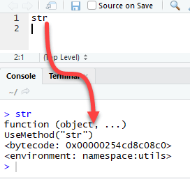
It is possible to see the source code of a function by running the name of the function itself in the console.
We will see three groups of function in action
General function
Maths function
Statistical function
General functions
We are already familiar with general functions like cbind(), rbind(),range(),sort(),order() functions. Each of these functions has a specific task, takes arguments to return an output.
Math functions
abs(x) |
Takes the absolute value of x |
log(x,base=y) |
Takes the logarithm of x with base y; if base is not specified, returns the natural logarithm |
exp(x) |
Returns the exponential of x |
sqrt(x) |
Returns the square root of x |
factorial(x) |
Returns the factorial of x (x!) |
Statistical functions
|
mean(x) |
Mean of x |
|
median(x) |
Median of x |
|
var(x) |
Variance of x |
|
sd(x) |
Standard deviation of x |
|
scale(x) |
Standard scores (z-scores) of x |
|
quantile(x) |
The quartiles of x |
|
summary(x) |
Summary of x: mean, min, max etc.. |
Write function in R
In some occasion, we need to write our own function because we have to accomplish a particular task and no ready made function exists. A user-defined function involves a name, arguments and a body
function.name <- function(arguments)
{
    computations on the arguments
    some other code
}
One argument function
we define a simple square function. The function accepts a value and returns the square of the value
square_function<- function(n)
{
  # compute the square of integer `n`
  n^2
}
# calling the function and passing value 4
square_function(4)
Code Explanation:
The function is named square_function; it can be called whatever we want.
It receives an argument "n". We didn't specify the type of variable so that the user can pass an integer, a vector or a matrix
-
The function takes the input "n" and returns the square of the input.
When you are done using the function, we can remove it with the rm() function.
rm(square_function)
square_function
Environment Scoping
In R, the environment is a collection of objects like functions, variables, data frame, etc.
The top-level environment available is the global environment, called R_GlobalEnv. And we have the local environment.
# List the content of the current environment
ls(environment())
Clarify the difference between global and local environment
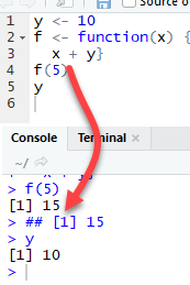
The function f returns the output 15. This is because y is defined in the global environment. Any variable defined in the global environment can be used locally. The variable y has the value of 10 during all function calls and is accessible at any time
Let's see what happens if the variable y is defined inside the function.
We need to drop `y` prior to run this code using rm r
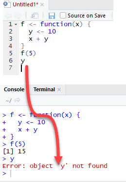
The output is also 15 when we call f(5) but returns an error when we try to print the value y. The variable y is not in the global environment.
Finally, R uses the most recent variable definition to pass inside the body of a function
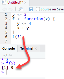
R ignores the y values defined outside the function because we explicitly created a y variable inside the body of the function.
We can write a function with more than one argument. Consider the function called "times". It is a straightforward function multiplying two variables.
Multi arguments function
times <- function(x,y) {
  x*y
	}
times(2,4)
When need to do many repetitive tasks
When should we write function?
Sometimes, we need to include conditions into a function to allow the code to return different outputs.
Functions with condition
# Example:
split_data <- function(df, train = TRUE)
# Arguments:
# -df: Define the dataset
# -train: Specify if the function returns the train set or test set. By default, set to TRUE
SQL in R
sqldf() from the package sqldf allows the use of SQLite queries to select and manipulate data in R
install.packages("sqldf")Control Structures in R
A control structure ‘controls’ the flow of code / commands written inside a function
-
IF, ELSE, ELSEIF Statement
-
For Loop
-
While Loop
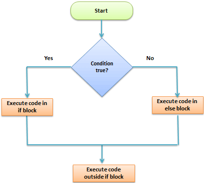
1. IF, ELSE, ELSEIF Statement
This structure is used to test a condition
if (<condition>){
         ##do something
} else {
         ##do something
}
The else if statement
We can further customize the control level with the else if statement. With else if, you can add as many conditions as we want
if (condition1) {
expr1
} else if (condition2) {
expr2
} else if (condition3) {
expr3
} else {
expr4
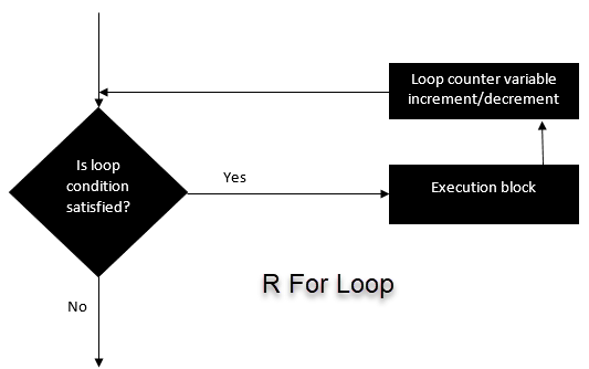
}2. For Loop
This structure is used when a loop is to be executed fixed number of times. It is commonly used for iterating over the elements of an object (list, vector)
for (i in vector){
          #do something
}
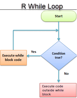
3. While Loop
It begins by testing a condition, and executes only if the condition is found to be true. Once the loop is executed, the condition is tested again
#initialize a condition
Age <- 12

#check if age is less than 17
while(Age < 17){
         print(Age)
         Age <- Age + 1 #Once the loop is executed, this code breaks the loop
}
apply(), sapply(), tapply() in R
The apply() family pertains to the R base package and is populated with functions to manipulate slices of data from matrices, arrays, lists and dataframes in a repetitive way. These functions allow crossing the data in a number of ways and avoid explicit use of loop constructs
apply() function
We use apply() over a matrice
apply(X, MARGIN, FUN)
# Here:
# -x: an array or matrix
# -MARGIN:  take a value or range between 1 and 2 to define where to apply the function:
# -MARGIN=1`: the manipulation is performed on rows
# -MARGIN=2`: the manipulation is performed on columns
# -MARGIN=c(1,2)` the manipulation is performed on rows and columns
# -FUN: tells which function to apply. Built functions like mean, median, sum, min, max and even user-defined functions can be applied>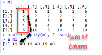
The code apply(m1, 2, sum) will apply the sum function to the matrix 5x6 and return the sum of each column accessible in the dataset
lapply() function
l in lapply() stands for list.
The difference between lapply() and apply() lies between the output return.
The output of lapply() is a list.
lapply() can be used for other objects like data frames and lists.
lapply() function does not need MARGIN.
lapply(X, FUN)
# Arguments:
# -X: A vector or an object
# -FUN: Function applied to each element of x
sapply() function
sapply() function does the same jobs as lapply() function but returns a vector.
sapply(X, FUN)
# Arguments:
# -X: A vector or an object
# -FUN: Function applied to each element of x
sapply() function is more efficient than lapply() in the output returned because sapply() store values direclty into a vector. But, it is not always the case.
Function |
Arguments |
Objective |
Input |
Output |
|---|---|---|---|---|
apply |
apply(x, MARGIN, FUN) |
Apply a function to the rows or columns or both |
Data frame or matrix |
vector, list, array |
lapply |
lapply(X, FUN) |
Apply a function to all the elements of the input |
List, vector or data frame |
list |
sapply |
sappy(X FUN) |
Apply a function to all the elements of the input |
List, vector or data frame |
vector or matrix |
We can use lapply() or sapply() interchangeable to slice a data frame
Slice vector
The function tapply() computes a measure (mean, median, min, max, etc..) or a function for each factor variable in a vector
tapply() Function
tapply(X, INDEX, FUN = NULL)
# Arguments:
# -X: An object, usually a vector
# -INDEX: A list containing factor
# -FUN: Function applied to each element of x
Summary
Mnemonics
- lapply is a list apply which acts on a list or vector and returns a list.
- sapply is a simple lapply (function defaults to returning a vector or matrix when possible)
- tapply is a tagged apply where the tags identify the subsets
- apply is generic: applies a function to a matrix's rows or columns (or, more generally, to dimensions of an array)
Import Data Into R
Data could exist in various formats. For each format R has a specific function and argument.
Read CSV
One of the most widely data store is the .csv (comma-separated values) file formats.
R loads an array of libraries during the start-up, including the utils package.
This package is convenient to open csv files combined with the reading.csv() function
read.csv(file, header = TRUE, sep = ",")
# argument:
# -file: PATH where the file is stored
# -header: confirm if the file has a header or not, by default, the header is set to TRUE
# -sep: the symbol used to split the variable. By default, `,`.
If your .csv file is stored locally, you can replace the PATH inside the code snippet. Don't forget to wrap it inside ' '. The PATH needs to be a string value.
read.csv(file, header = TRUE, sep = ",")
# argument:
# -file: PATH where the file is stored
# -header: confirm if the file has a header or not, by default, the header is set to TRUE
# -sep: the symbol used to split the variable. By default, `,`.
Excel files are very popular among data analysts. Spreadsheets are easy to work with and flexible. R is equipped with a library readxl to import Excel spreadsheet
Read Excel Files
read_excel(PATH, sheet = NULL, range= NULL, col_names = TRUE)
# arguments:
# -PATH: Path where the excel is located
# -sheet: Select the sheet to import. By default, all
# -range: Select the range to import. By default, all non-null cells
# -col_names: Select the columns to import. By default, all non-null columns
We can find out which sheets are available in the workbook by using excel_sheets() function
excel_sheets()
Use n_max argument to return n rows
Use range argument combined with cell_rows or cell_cols
control cells to read in 2 ways
# Read the first five row: with header
iris <-read_excel(example, n_max =5, col_names =TRUE)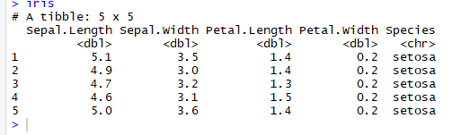
n_max argument to return n rows
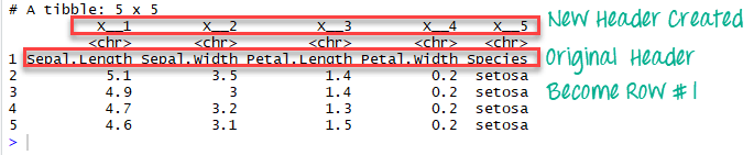
If we change col_names to FALSE, R creates the headers automatically
# Read the first five row: without header
iris_no_header <-read_excel(example, n_max =5, col_names =FALSE)
In the data frame iris_no_header, R created five new variables named
X__1, X__2, X__3, X__4 and X__5
Range argument combined with cell_rows or cell_cols
# Read rows A1 to B5
example_1 <-read_excel(example, range = "A1:B5", col_names =TRUE)
dim(example_1)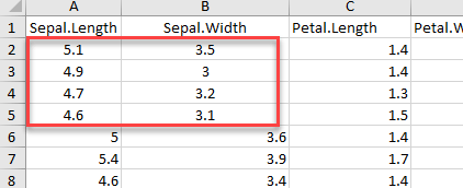
Use the function cell_rows() which controls the range of rows to return
# Read rows 1 to 5
example_2 <-read_excel(example, range =cell_rows(1:5),col_names =TRUE)
dim(example_2)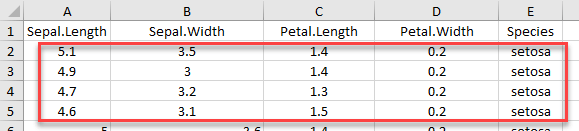
If we want to import rows which do not begin at the first row, we have to include col_names = FALSE
iris_row_with_header <-read_excel(example, range =cell_rows(2:3), col_names=TRUE)
iris_row_no_header <-read_excel(example, range =cell_rows(2:3),col_names =FALSE)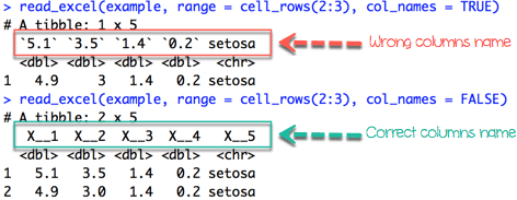
cell_cols() select the columns with the letter.
# Select columns A and B
col <-read_excel(example, range =cell_cols("A:B"))
dim(col)
read_excel() returns NA when a symbol without numerical value appears in the cell. We can count the number of missing values with the combination of two functions
sum
is.na
iris_na <-read_excel(example, na ="setosa")
sum(is.na(iris_na))
Load Data From Database
There are various R packages that can be used to communicate with RDBMS, each with a different level of abstraction.
Some of these packages have the functionality of copying entire data frames to and from databases.
-
Some of the packages available on CRAN for importing data from Relational Database are:
RMySQL/RMariaDB
RODBC
ROracle
RPostgreSQL
RSQLite (This packages is used for bundled DBMS SQLite)
RJDBC (This package uses Java and can connect to any DBMS with a JDBC driver)
PL/R
RpgSQL
RMongo (This is an R interface for Java Client with MongoDB)
Using RMySQL()/RMariaDB()
RMySQL package is an interface to MySQL DBMS. The current version of this package requires DBI package to be pre-installed
dbGetQuery sends the queries and fetches results as the data frame.
dbSendQuery only sends the query and returns an object of class inheriting from “DBIResult”, this object of class can be used to fetch the required result.
dbClearResult removes the result from cache memory.
fetch returns few or all rows that were asked in query. The output of fetch function is a list.
dbHasCompleted is used to check is all the rows are retrieved.
dbReadTable and dbWriteTable functions are used to read and write the tables in Database from an R data frame.
Best practices for Data Import
When we want to import data into R, it is useful to implement following checklist. It will make it easy to import data correctly into R
The typical format for a spreadsheet is to use the first rows as the header (usually variables name).
Avoid to name a dataset with blank spaces; it can lead to interpreting as a separate variable. Alternatively, prefer to use '_' or '-.'
Short names are preferred
Do not include symbol in the name: i.e: exchange_rate_$_€ is not correct. Prefer to name it: exchange_rate_dollar_euro
Use NA for missing values otherwise; we need to clean the format later.
|
utils |
Read CSV file |
read.csv() |
file, header =,TRUE, sep = "," |
|
readxl |
Read EXCEL file |
read_excel() |
path, range = NULL, col_names = TRUE |
|
haven |
Read SAS file |
read_sas() |
path |
|
haven |
Read STATA file |
read_stata() |
path |
|
haven |
Read SPSS fille |
read_sav() |
path |
Library
Objective
Function
Default Arguments
Summary
|
read_excel() |
Read n number of rows |
n_max = 10 |
|
Select rows and columns like in excel |
range = "A1:D10" |
|
|
Select rows with indexes |
range= cell_rows(1:3) |
|
|
Select columns with letters |
range = cell_cols("A:C") |
Function
Objectives
Arguments
Replace Missing Values
Missing values in data science arise when an observation is missing in a column of a data frame or contains a character value instead of numeric value. Missing values must be dropped or replaced in order to draw correct conclusion from the data
mutate()
The fourth verb in the dplyr library is helpful to create new variable or change the values of an existing variable.
We will proceed in two parts. We will learn how to:
- exclude missing values from a data frame
- impute missing values with the mean and median
mutate(df, name_variable_1 = condition, ...)
# arguments:
# -df: Data frame used to create a new variable
# -name_variable_1: Name and the formula to create the new variable
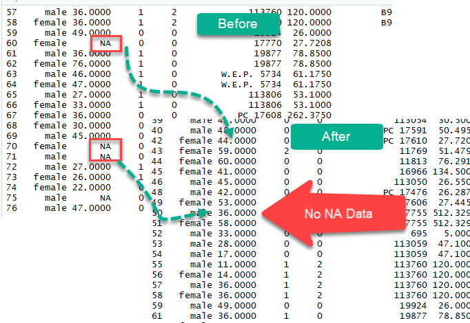
# -...: No limit constraint. Possibility to create more than one variable inside mutate()Exclude Missing Values (NA)
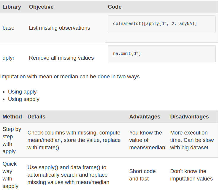
The na.omit() method from the dplyr library is a simple way to exclude missing observation. Dropping all the NA from the data is easy but it does not mean it is the most elegant solution. During analysis, it is wise to use variety of methods to deal with missing values
Impute missing values (NA)
We could also impute(populate) missing values with the median or the mean. A good practice is to create two separate variables for the mean and the median. Once created, we can replace the missing values with the newly formed variables
Use the apply method to compute the mean of the column with NA
- Earlier, we stored the columns name with the missing values in the list called list_na. We will use this list
- Now we need to compute of the mean with the argument na.rm = TRUE. This argument is compulsory because the columns have missing values, and this tells R to ignore them.
- Replace the NA Values
- We can replace the missing observations with the median as well.
- A big data set could have lots of missing values and the above method could be cumbersome. We can execute all the above steps above in one line of code using sapply() method
Summary
We have three methods to deal with missing values:
- Exclude all of the missing observations
- Impute with the mean
- Impute with the median
Exporting Data
How to Export Data from R
To export data to the hard drive, we need the file path and an extension.
- First of all, the path is the location where the data will be stored. We will store data on:
- The Hard Drive
- Google Drive
- Secondly, we will export the data into different types of files, such as:
- csv
- xlsx
Export to Hard drive
save the data directly into the working directory
directory <-getwd()
directory
Export CSV
write.csv(df, path)
# arguments
# -df: Dataset to save. Need to be the same name of the data frame in the environment.
# -path: A string. Set the destination path. Path + filename + extension i.e. "/Users/USERNAME/Downloads/mydata.csv" or the filename + extension if the folder is the same as the working directory
Export to Excel file
library(xlsx)
write.xlsx(df, "file-name.xlsx")
the library xlsx uses Java to create the file. Java needs to be installed if not present in your machine
Save RData
save(x,file-name)
# arguments:
# x = Variable
# file-name = File name ".RData"
Save a data frame or any other R object, using save() function
Interact With
Google Drive
install.packages("googledrive") Install googledrive library to access the function allowing to interact with Google Drive
Upload to
Google Drive
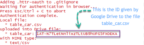
drive_upload(file, path = NULL, name = NULL)
# arguments:
# - file: Full name of the file to upload (i.e., including the extension)
# - path: Location of the file- name: You can rename it as you wish. By default, it is the local name.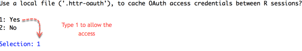
- Then, you are redirected to Google API to allow the access. Click Allow.
- Once the authentication is complete, you can quit your browser.
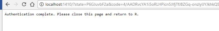
In the Rstudio's console, you can see the summary of the step done. Google successfully uploaded the file located locally on the Drive. Google assigned an ID to each file in the drive.
View file in Google Spreadsheet
drive_browse("table_car")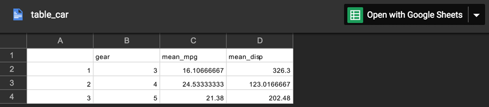
Import from Google Drive
drive_download(file, path = NULL, overwrite = FALSE)
# arguments:
# - file:  Name or id of the file to download
# -path: Location to download the file. By default, it is downloaded to the working directory and the name as in Google Drive
# -overwrite = FALSE: If the file already exists, don't overwrite it. If set to TRUE, the old file is erased and replaced by the new one.
Upload a file from Google Drive with the ID is convenient. We can get the ID by the file name
|
base |
Export csv |
write.csv() |
|
xlsx |
Export excel |
write.xlsx() |
|
haven |
Export spss |
write_sav() |
|
haven |
Export sas |
write_sas() |
|
haven |
Export stata |
write_dta() |
|
base |
Export R |
save() |
|
googledrive |
Upload Google Drive |
drive_upload() |
|
googledrive |
Open in Google Drive |
drive_browse() |
|
googledrive |
Retrieve file ID |
drive_get(as_id()) |
|
googledrive |
Dowload from Google Drive |
download_google() |
|
googledrive |
Remove file from Google Drive |
drive_rm() |
|
rdrop2 |
Authentification |
drop_auth() |
|
rdrop2 |
Create a folder |
drop_create() |
|
rdrop2 |
Upload to Dropbox |
drop_upload() |
|
rdrop2 |
Read csv from Dropbox |
drop_read_csv |
|
rdrop2 |
Delete file from Dropbox |
drop_delete() |
Library
Objective
Function
R Aggregate Function
Summary of a variable is important to have an idea about the data
Before we perform summary, we will do the following steps to prepare the data:
- Step 1: Import the data
- Step 2: Select the relevant variables
- Step 3: Sort the data
Use the glimpse() function to have an idea about the structure of the dataset
Summarise()
The syntax of summarise() is basic and consistent with the other verbs included in the dplyr library
summarise(df, variable_name=condition)
# arguments:
# - `df`: Dataset used to construct the summary statistics
# - `variable_name=condition`: Formula to create the new variable
Group_by
vs
no group_by
group_by works perfectly with all the other verbs (i.e. mutate(), filter(), arrange(), ...)
Combining group_by(), summarise() and ggplot() together
- Step 1: Select data frame
- Step 2: Group data
- Step 3: Summarize the data
- Step 4: Plot the summary statistics
Function in summarise()
|
Basic |
mean() |
Average of vector x |
|
|
median() |
Median of vector x |
|
|
sum() |
Sum of vector x |
|
variation |
sd() |
standard deviation of vector x |
|
|
IQR() |
Interquartile of vector x |
|
Range |
min() |
Minimum of vector x |
|
|
max() |
Maximum of vector x |
|
|
quantile() |
Quantile of vector x |
|
Position |
first() |
Use with group_by() First observation of the group |
|
|
last() |
Use with group_by(). Last observation of the group |
|
|
nth() |
Use with group_by(). nth observation of the group |
|
Count |
n() |
Use with group_by(). Count the number of rows |
|
|
n_distinct() |
Use with group_by(). Count the number of distinct observations |
Objective
Function
Description
Basic function
Subsetting
The function summarise() is compatible with subsetting.
Sum
Another useful function to aggregate the variable is sum().
Standard deviation
Spread in the data is computed with the standard deviation or sd() in R
Minimum and maximum
Access the minimum and the maximum of a vector with the function min() and max().
Count
Count observations by group is always a good idea. With R, we can aggregate the the number of occurence with n()
First and last
Select the first, last or nth position of a group
nth observation
The function nth() is complementary to first() and last(). We can access the nth observation within a group with the index to return
Distinct number of observation
The function n() returns the number of observations in a current group. A closed function to n() is n_distinct(), which count the number of unique values
Multiple groups
A summary statistic can be realized among multiple groups
Filter
Before we intend to do an operation, we can filter the dataset
Ungroup
We need to remove the grouping before we want to change the level of the computation
R Select(), Filter(), Arrange(), Pipeline
select()
We don't necessarily need all the variables, and a good practice is to select only the variables you find relevant
#- `select(df, A, B ,C)`: Select the variables A, B and C from df dataset.
#- `select(df, A:C)`: Select all variables from A to C from df dataset.
#- `select(df, -C)`: Exclude C from the dataset from df dataset.
Filter()
The filter() verb helps to keep the observations following a criteria
filter(df, condition)
# arguments:
# - df: dataset used to filter the data
# - condition:  Condition used to filter the data
Pipeline
The creation of a dataset requires a lot of operations, such as:
- importing
- merging
- selecting
- filtering
- and so on
The dplyr library comes with a practical operator, %>%, called the pipeline. The pipeline feature makes the manipulation clean, fast and less prompt to error
arrange()
The arrange() verb can reorder one or many rows, either ascending (default) or descending
# - `arrange(A)`: Ascending sort of variable A
# - `arrange(A, B)`: Ascending sort of variable A and B
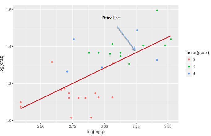
# - `arrange(desc(A), B)`: Descending sort of variable A and ascending sort of B Scatter plot with ggplot2
Graphs are an incredible tool to simplify complex analysis
Graphs are the third part of the process of data analysis. The first part is about data extraction, the second part deals with cleaning and manipulating the data. At last, we need to visualize our results graphically.
ggplot2 package
ggplot2 is very flexible, incorporates many themes and plot specification at a high level of abstraction. With ggplot2, we can't plot 3-dimensional graphics and create interactive graphics
The basic syntax of ggplot2 is:
ggplot(data, mapping=aes()) +
geometric object
# arguments:
# data: Dataset used to plot the graph
# mapping: Control the x and y-axis
# geometric object: The type of plot you want to show. The most common object are:
# - Point: `geom_point()`
# - Bar: `geom_bar()`
# - Line: `geom_line()`
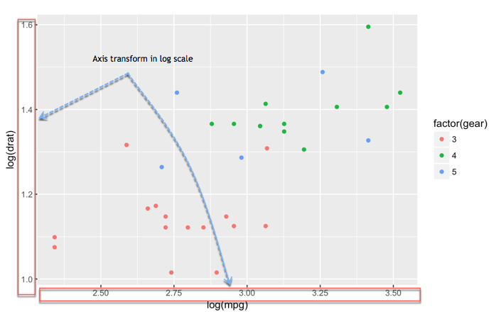
# - Histogram: `geom_histogram()`Change axis
One solution to make our data less sensitive to outliers is to rescale them
Scatter plot with fitted values
We can add another level of information to the graph. We can plot the fitted value of a linear regression.
Add information to the graph
Graphs need to be informative and good labels. We can add labels with labs()function
lab(title = "Hello Fathi")
# argument:
# - title: Control the title. It is possible to change or add title with:
# - subtitle: Add subtitle below title
# - caption: Add caption below the graph
# - x: rename x-axis
# - y: rename y-axis
# Example:lab(title = "Hello Fathi", subtitle = "My first plot")
Theme
The library ggplot2 includes eights themes:
- theme_bw()
- theme_light()
- theme_classis()
- theme_linedraw()
- theme_dark()
- theme_minimal()
- theme_gray()
- theme_void()
Save Plots
ggsave("my_fantastic_plot.png")Store graph right after we plot it
How to make Boxplot in R
Box plot helps to visualize the distribution of the data by quartile and detect the presence of outliers
Hands On Tutorial in RStudio
Bar Chart & Histogram
Bar chart is a great way to display categorical variables in the x-axis. This type of graph denotes two aspects in the y-axis.
- The first one counts the number of occurrence between groups.
- The second one shows a summary statistic (min, max, average, and so on) of a variable in the y-axis
How to create Bar Chart
ggplot(data, mapping = aes()) +
geometric object

# arguments:
# data: dataset used to plot the graph
# mapping: Control the x and y-axis
# geometric object: The type of plot you want to show. The most common objects are:

# - Point: `geom_point()`
# - Bar: `geom_bar()`
# - Line: `geom_line()`
# - Histogram: `geom_histogram()`
Customize the graph
# - `stat`: Control the type of formatting. By default, `bin` to plot a count in the y-axis. For continuous value, pass `stat = "identity"`
# - `alpha`: Control density of the color
# - `fill`: Change the color of the bar
# - `size`: Control the size the bar
Four arguments can be passed to customize the graph
Hands On Tutorial in RStudio
Histogram
Represent the group of variables with values in the y-axis
R Interactive Map (leaflet)
Leaflet is one of the most popular open-source JavaScript libraries for interactive maps
Leaflet Package
install.packages("leaflet")
# to install the development version from Github, run
# devtools::install_github("rstudio/leaflet")
Hands On Tutorial in RStudio
R Markdown
R Markdown is a simple formatting syntax for authoring HTML, PDF, and MS Word documents
For more details on using R Markdown see http://rmarkdown.rstudio.com.
Some advantages of using R Markdown:
-
R code can be embedded in the report, so it is not necessary to keep the report and R script separately. Including the R code directly in a report provides structure to analyses.
-
The report text is written as normal text, so no knowledge of HTML coding is required.
-
The output is an HTML file that includes pictures, code blocks R output and text. No additional files are needed, everything is incorporated in the HTML file. So easy to send the report via mail, or place it as paper package on your website.
-
These HTML reports enhance collaboration: It is much more easy to comment on an analysis when the R code, the R output and the plots are available in the report.
How to generate an HTML report
Open R Studio, then go to
File →→ New file →→ R Markdown.
Emphasis
*italic*
**bold**
_italic_
__bold__
Headers
# Header 1
## Header 2
### Header 3
#### Header 4
##### Header 5
###### Header 6
List - Ordered List
1. Item 1
2. Item 2
3. Item 3
+ Item 3a
+ Item 3b
List - Unordered List
* Item 1
* Item 2
+ Item 2a
+ Item 2b
R Code Chucks
```{r}

summary(cars$dist)

summary(cars$speed)

```
Inline R Code
There were `r nrow(cars)` cars studiedBlockquotes
> Put some quote hereLinks
[title](http://www.google.com)Plain Code Blocks
```

Some text here

```
Table Output
knitr::kable(dataset)Include Image
!Fotia Logo](img/logo kuda-01.png)```{r fig.width=1, fig.height=10,echo=FALSE}
library(png)
library(grid)
img <- readPNG("img/logo kuda-01.png")
grid.raster(img)
```Resize Image
Argument in Code Chunk
The argument echo specifies whether the R commands are included (default is TRUE). Adding echo=FALSE in the opening line of the R code block will not include the commmand:
```{r, echo=FALSE}
- The argument eval specifies whether the R commands is evaluated (default is TRUE). Adding eval=FALSE in the opening line of the R code block will not evaluate the commmand: ```{r, eval=FALSE}. Now only the command is shown, but no output.
- The argument include specifies whether the output is included (default is TRUE). Adding include=FALSE in the opening line of the R code block will not include the commmand: ```{r, include=FALSE}. Now the command and the output are both not shown, but the statement is evaluated.
It is good practice to provide a name for each R code block, which helps with debugging. Add a name nameblock directly behind the r:
```{r nameblock, echo=FALSE}. Note that the name should be unique.
Embedding plots with specific size
```{r plot2, fig.width = 8, fig.height = 4, echo=FALSE}
    par(mfrow(1,3))
    plot(cars)
    image(volcano, col.terrain.colors(50))
```
Note that the echo = FALSE parameter was added to the code chunk to prevent printing of the R code that generated the plot
Although no HTML coding is required, HTML could optionally be used to format the report. The HTML tags are interpreted by the browser after the .Rmd file is converted into an HTML file. Some examples:
- color word: <span style="color:red">color</span> word
- mark word: <span style="background:yellow">mark</span> word
- quick way of adding more space after text block: <p></br></p>
R Shiny Dashboard
Shiny is a means of creating web applications entirely in R.
The client-server communication, HTML, layout and JavaScript programming is entirely handled by Shiny.
This makes creating web applications feasible for those who are not necessarily experienced web-developers
Package Shinydashboard
install.packages("shinydashboard")
library(shinydashboard)
Basics
## ui.R ##
library(shinydashboard)

dashboardPage(
  dashboardHeader(),
  dashboardSidebar(),
  dashboardBody()
)
A dashboard has three parts:
a header, a sidebar, and a body.
shinyapp()
## app.R ##
library(shiny)
library(shinydashboard)

ui <- dashboardPage(
  dashboardHeader(),
  dashboardSidebar(),
  dashboardBody()
)

server <- function(input, output) { }

shinyApp(ui, server)
HEADER
dashboardHeader(title = "My Dashboard")Setting the title is simple;
just use the title argument
Sidebar menu items and tabs
Links in the sidebar can be used like tabPanels from Shiny. That is, when we click on a link, it will display different content in the body of the dashboard.
## ui.R ##
sidebar <- dashboardSidebar(
  sidebarMenu(
    menuItem("Dashboard", tabName = "dashboard", icon = icon("dashboard")),
    menuItem("Widgets", icon = icon("th"), tabName = "widgets",
             badgeLabel = "new", badgeColor = "green")
  )
)

body <- dashboardBody(
  tabItems(
    tabItem(tabName = "dashboard",
      h2("Dashboard tab content")
    ),

    tabItem(tabName = "widgets",
      h2("Widgets tab content")
    )
  )
)

# Put them together into a dashboardPage
dashboardPage(
  dashboardHeader(title = "Simple tabs"),
  sidebar,
  body
)CHEATSHEET
There are no secrets to success. It is the result of preparation, hard work, and learning from failure. - Colin Powell
THANK YOU
R Programming (Training)
By Abdullah Fathi
R Programming (Training)
R Programming Training Basic


