Machine Learning
Abdullah Fathi


Introduction
- Machine learning is a subset of artificial intelligence.
- Focuses mainly on designing systems which allow them to learn and make predictions based on some experience which is data.

Machine learning is becoming widespread among data scientist and is deployed in hundreds of products we use daily. One of the first ML application was spam filter
Applications of ML

Applications of ML

Supervised
VS
Unsupervised
Supervised Learning
Training data feed to the algorithm includes a label (answer)
-
Classification
- Most used supervised learning technique
-
Regressions
- Commonly used in ML field to predict continuous value.
- Predict the value of dependant variable based on a set of independant variables (also called predictors or regressors)
Lists of some fundamental supervised learning algorithms
- Linear Regression
- Logistic Regression
- Neares Neighbours
- Support Vector Machine (SVM)
- Decision trees and Random Forest
- Neural Networks
Unsupervised Learning
Training data is unlabeled.
The system tries to learn without a reference
List of unsupervised learning algorithms
- K-mean
- Hierarchical Cluster Analysis
- Expectation Maximization
- Visualization and dimensionality reduction
- Principal Component Analysis
- Kernel PCA
- Locally-Linear Embedding
- Data PreProcessing
-
Regression
- Simple Linear Regression
- Multiple Linear Regression
- Polynomial Regression
- Support Vector Regression (SVR)
- Decision Tree Regression
- Random Forest Regression
- Evaluating Regression Model Performance
-
Classification
- Logistic Regression
- K-Nearest Neighbour (KNN)
- Support Vector Machine (SVM)
- Kernel SVM
- Naive Bayes
- Decision Tree Classification
- Random Forest Classification
- Evaluating Classification Models Performance
-
Clustering
- K-Means Clustering
- Hierarchical Clustering
-
Association Rule Learning
- Apriori
- Eclat
-
Reinforcement Learning
- Upper Confidence Bound (UCB)
- Thompson Sampling
- Natural Language Processing (NLP)
-
Deep Learning
- Artificial Neural Network
-
Dimensionality Reduction
- Principal Component Analysis (PCA)
- Linear Discriminant Analysis (LDA)
- Kernel PCA
-
Model Selection
- K-Fold Cross Validation
- Grid Search
- XGBoost
Data Preprocessing
Before begin our journey with machine learning, we need to prepare our data
Regression
Regression models (both linear and non-linear) are used for predicting a real value, like salary for example. If our independent variable is time, then we are forecasting future values, otherwise our model is predicting present but unknown values. Regression technique vary from Linear Regression to SVR and Random Forests Regression
ML Regression Models
- Simple Linear Regression
- Multiple Linear Regression
- Polynomial Regression
- Support Vector for Regression (SVR)
- Decision Tree Classification
- Random Forest Classification
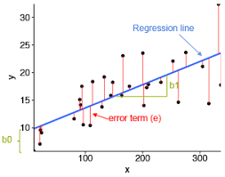
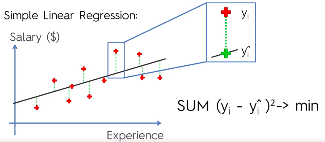
Simple Linear Regression

Simple Linear Regression
y = Dependant Variable (DV)
X = Independant Variable (IV)
b1 = Coefficient
b0 = Constant
lm(formula, data)

# Where
#    formula = A symbolic description of the model to be fitted
#    data = An optional data frame
Multiple Linear Regression

Assumptions of a Linear Regression
- Linearity
- Homoscedasticity
- Multivariate Normality
- Independence of Errors
- Lack of Multicollinearity

Building a Model
Building a Model

Building a Model
5 methods of building models:
- All-in
- Backward Elimination
- Forward Selection
- Bidirectional Elimination
- Score Comparison
Stepwise Regression: Backward Elimination, Forward Selection, Bidirectional Elimination
Method 1:
"All-in"
- Prior knowledge; OR
- You have to; OR
- Preparing for Backward Elimination
Method 2:
Backward Elimination
STEP 1: Select a significance level to stay in the model
(ex: Significance Level (SL) = 0.05)
STEP 2: Fit the full model with all possible predictors (independant variable)
STEP 3: Consider the predictor with the highest P-value. If P > Significance Level (SL), go to STEP 4, otherwise go to FIN
STEP 4: Remove the predictor
STEP 5: Fit model without this variable*
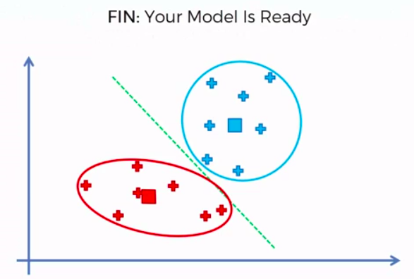
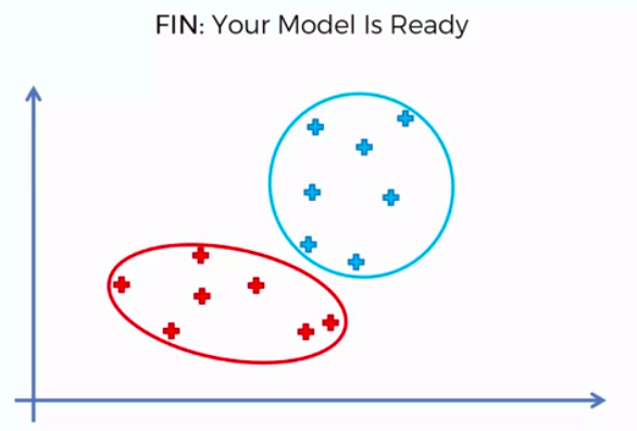
FIN: Our Model is Ready
Method 3:
Forward Selection
STEP 1: Select a significance level to enter the model
(ex: SL = 0.05)
STEP 2: Fit all simple regression models y ~ Xn Select the one with the lowest P-value
STEP 3: Keep this variable and fit all possible models with one extra predictor added to the one(s) we already have
STEP 4: Consider the predictor with the lowest P-value.
If P < SL, go to STEP 3, otherwise go to FIN
FIN: Keep the previous model
Method 4:
Bidirectional Elimination
STEP 1: Select a significance level to enter and to stay in the model (ex: SLENTER = 0.05, SLSTAY = 0.05)
STEP 2: Perform the next step of Forward Selection (new variables must have: P < SLENTER to enter)
STEP 3: Perform ALL steps of Backward Elimination (old variables must have P < SLSTAY to stay)
STEP 4: Now new variables can enter and no old variables can exit
FIN: Our Model is Ready
Method 5:
All Possible Models
STEP 1: Select a criterion of goodness of fit
(ex: Akaike criterion)
STEP 2: Construct All Possible Regression Model:
2^n - 1 total combinations
STEP 3: Select the one with the best criterion
FIN: Our Model is Ready
Ex:
10 columns means
1,023 models
Polynomial Linear Regression


b2X1^2 - give parabolic effect to fit our data better
Polynomial Linear Regression is a special case of Multiple Linear Regression
Support Vector Regression (SVR)
- Kernel: The function used to map a lower dimensional data into a higher dimensional data.
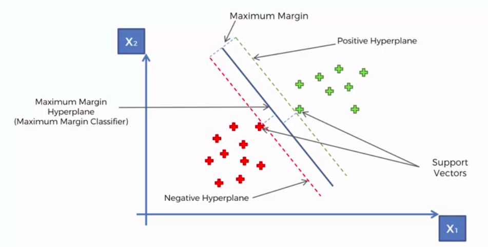
- Hyper Plane: In SVM this is basically the separation line between the data classes. Although in SVR we are going to define it as the line that will will help us predict the continuous value or target value
- Boundary line: In SVM there are two lines other than Hyper Plane which creates a margin . The support vectors can be on the Boundary lines or outside it. This boundary line separates the two classes. In SVR the concept is same.
- Support vectors: This are the data points which are closest to the boundary. The distance of the points is minimum or least.
TERMS
- Support Vector Machines support linear and nonlinear regression that we can refer to as SVR
- Instead of trying to fit the largest possible street between two classes while limiting margins violation, SVR tries to fit as many instances as possible on the street while limiting margins violations.
- The width of the street is controlled by a hyper parameter Epsilon
- SVR performs linear regression in a higher (dimensional space).
- We can think of SVR as if each data point in the training represents it's own dimension. When we evaluate our kernel between a test point and a point in the training set, the resulting value gives us the coordinate of our test point in that dimension.
- The vector we get when we evaluate the test point for all points in the training set, (k vector) is the representation of the test point in the higher dimensional space.
- Once we have that vector, we use it to perform linear regression
Building a SVR
- Collect a training set t = {X, Y}
- Choose a kernel and it's parameters as well as any regularization needed.
- Form the correlation matrix, K
- Train our machine, exactly or approximately, to get contraction coefficients a = {ai}
- Use those coefficients, create our estimator f(X,a,x) = y
Next step is to choose kernel
- Gaussian
Regularization
- Noise
SVR has a different regression goal compared to linear regression. In linear regression we are trying to minimize the error between the prediction and data. In SVR our goal is to make sure that errors do not exceed the threshold

Decision boundary is our Margin of tolerance that is We are going to take only those points who are within this boundary.
Or in simple terms that we are going to take only those those points which have least error rate. Thus giving us a better fitting model.
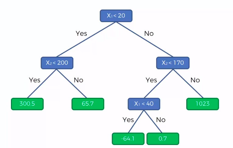
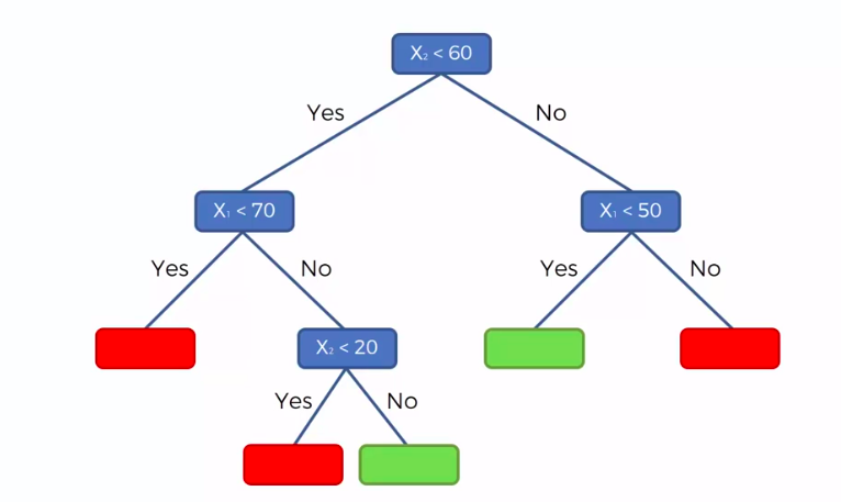
Decision Tree Regression
CART
Classification And Regression Trees
Classification Trees
Regression
Trees
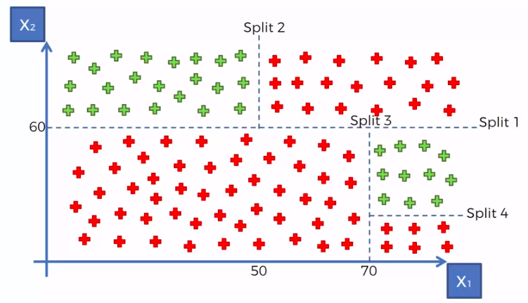
X1 and X2 is Independent Variable
Y is our Dependent Variable which we could not see because it is in another dimension (z-axis)
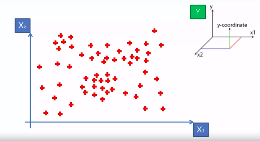
- Scatter plot will be split up into segment
- Split is determine by the algorithm.
- It is actually involve looking at something called information entropy
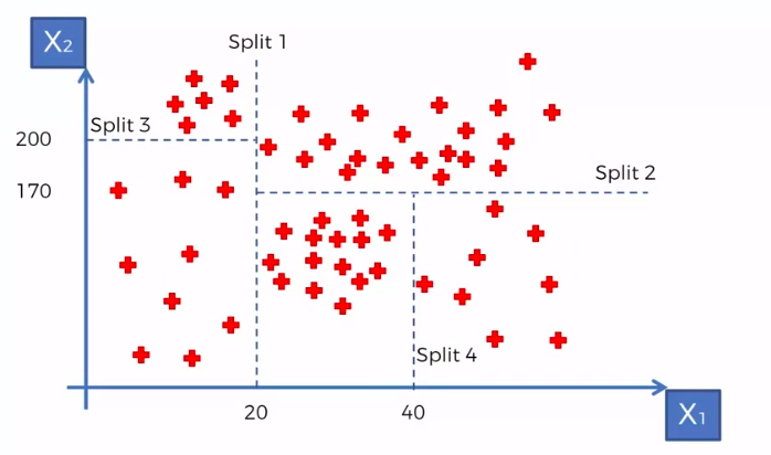
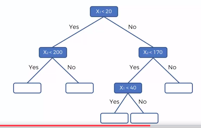
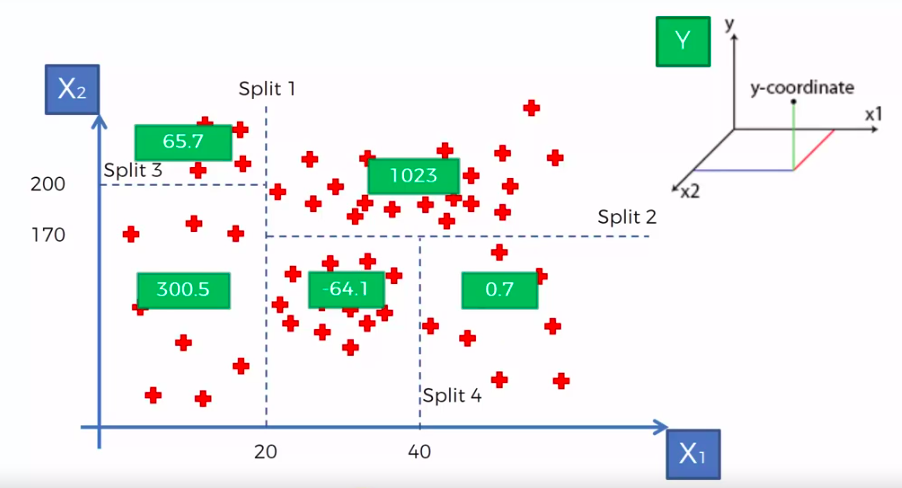
Calculate Mean/Average for each leaf
Random Forest Regression
Random Forest
STEP 1: Pick at random K data points from the Training set.
STEP 2: Build the tree associated to these K data points.
STEP 3: Choose the number Ntree of trees we want to build and repeat STEPS1 & 2
STEP 4: For a new data point, make each one of your Ntree trees predict value of Y to for the data point in question, and assign the new data point the average across all of the predicted Y values.
We are not just predicting based on 1 Tree, We are predicting based on forest of trees. It will improve the accuracy of prediction because we take the average of many prediction
Ensemble training is more stable because one changes of data could really impact one tree, but to impact a forest of trees it would be much harder
Ensemble Training

R-Squared

Adjusted R-Squared


Evaluating Regression Model Performance

Interpreting Linear Regression Coefficients

Pros and the Cons of each regression model

Classification
Unlike regression where we predict a continuous number, we use classification to predict a category. There is a wide variety of classification applications from medicine to marketing. Classification models include linear models like Logistic Regression, SVM, and nonlinear ones like K-NN, Kernel SVM and Random Forests
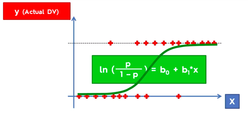
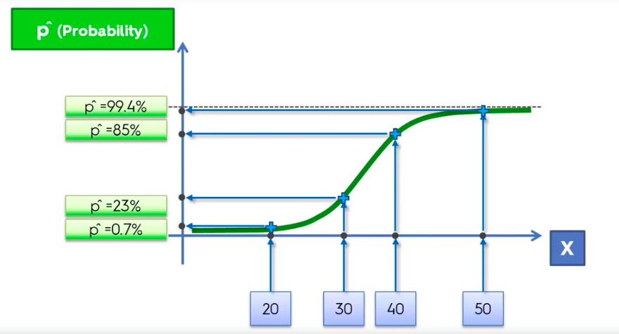
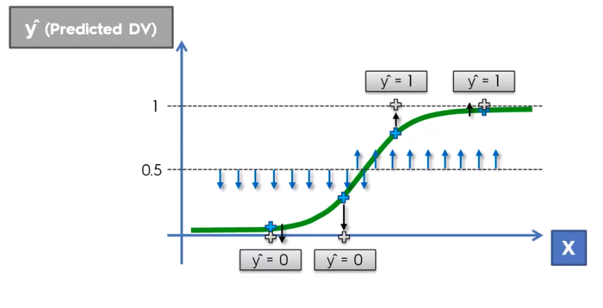
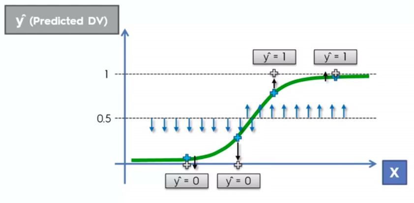
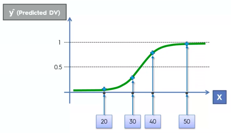
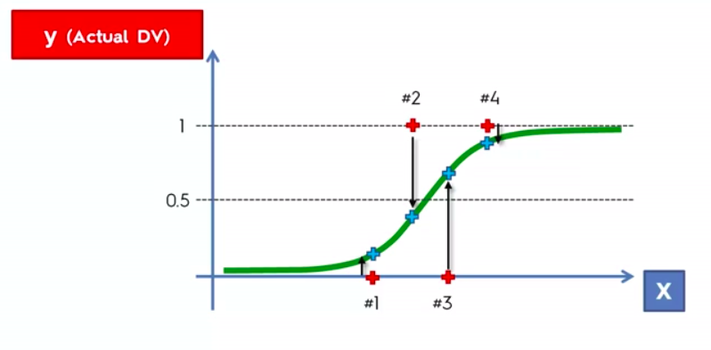
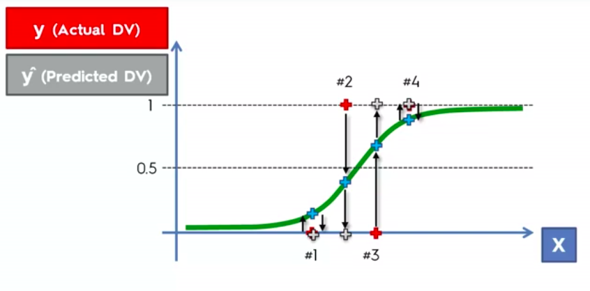
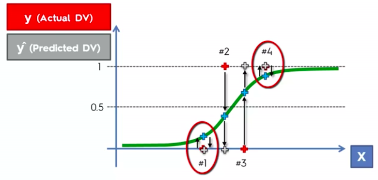
Logistic Regression
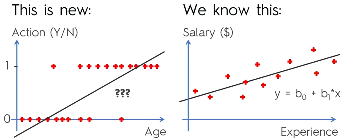
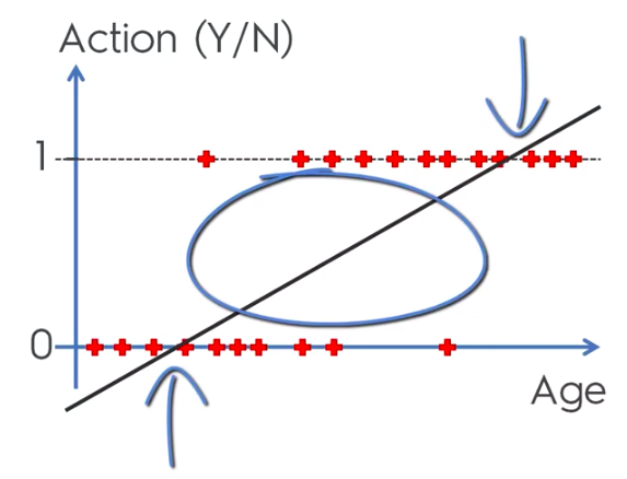
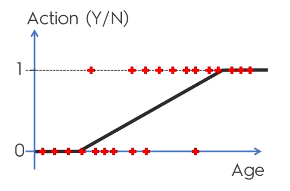
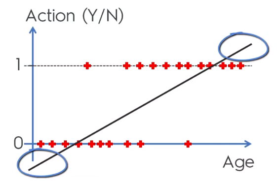
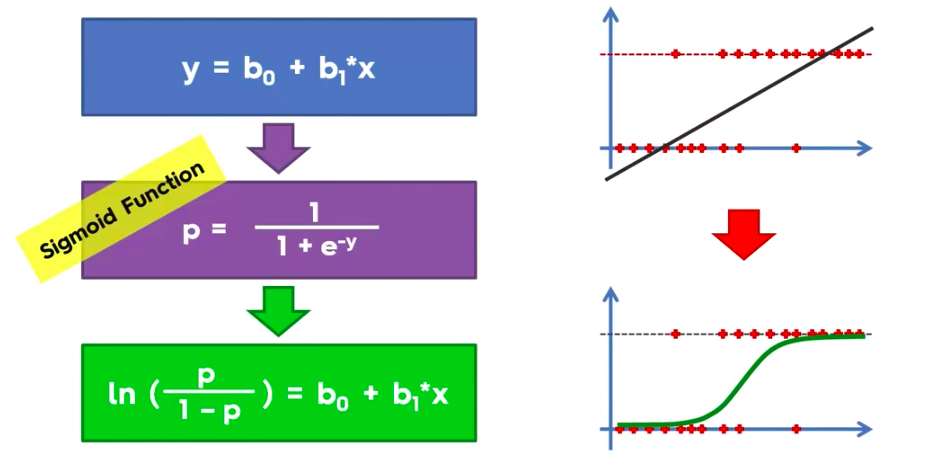
Logistic Regression Equation
library(ElemStatLearn)
set = training_set
X1 = seq(min(set[, 1]) - 1, max(set[, 1]) + 1, by = 0.01)
X2 = seq(min(set[, 2]) - 1, max(set[, 2]) + 1, by = 0.01)
grid_set = expand.grid(X1, X2)
colnames(grid_set) = c('Age', 'EstimatedSalary')
prob_set = predict(classifier, type = 'response', newdata = grid_set)
y_grid = ifelse(prob_set > 0.5, 1, 0)
plot(set[, -3],
     main = 'Logistic Regression (Training set)',
     xlab = 'Age', ylab = 'Estimated Salary',
     xlim = range(X1), ylim = range(X2))
contour(X1, X2, matrix(as.numeric(y_grid), length(X1), length(X2)), add = TRUE)
points(grid_set, pch = '.', col = ifelse(y_grid == 1, 'springgreen3', 'tomato'))
points(set, pch = 21, bg = ifelse(set[, 3] == 1, 'green4', 'red3'))
Visualizing The Results
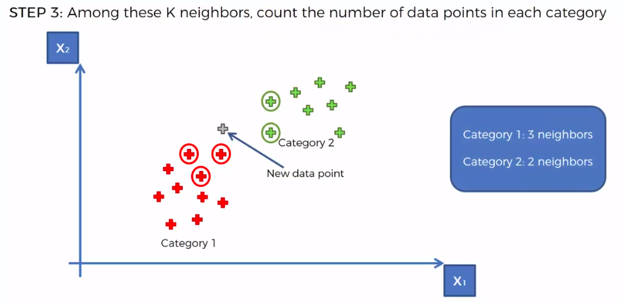
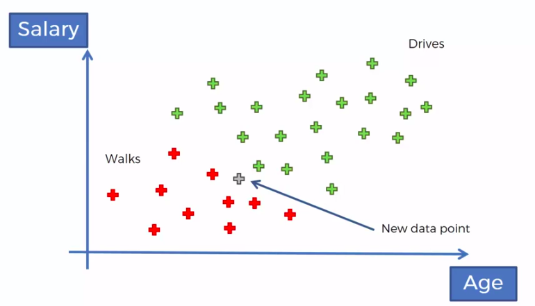
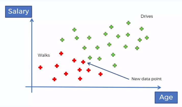
K-Nearest Neighbour
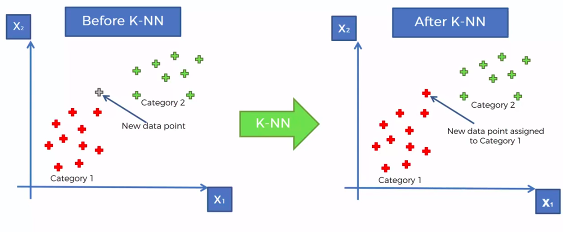
KNN
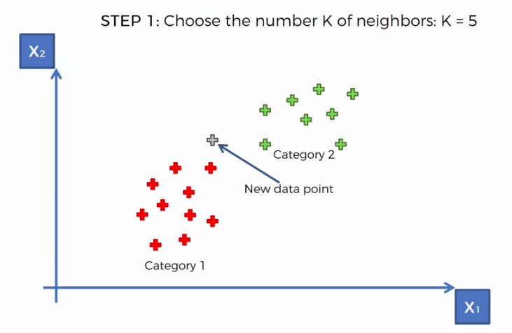
STEP 1: Choose the number K of neighbours
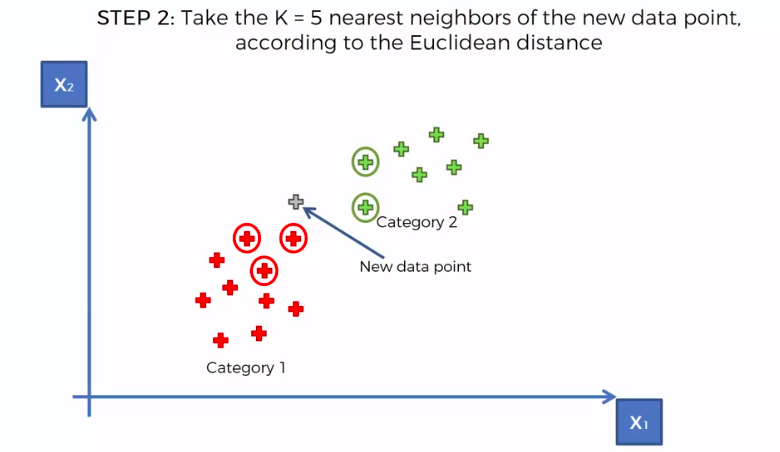
STEP 2: Take the K nearest neighbors of the new data point, according to the Euclidean distance
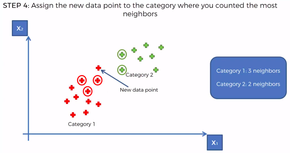
STEP 3: Among these K neighbors, count the number of data points in each category
STEP 4: Assign the new data point to the category where you counted the most neighbours
FIN: Our Model is Ready
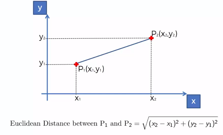
We can use other Distance as well such as Manhattan Distance. But Euclidean is the commonly used for geometry
Support Vector Machine (SVM)
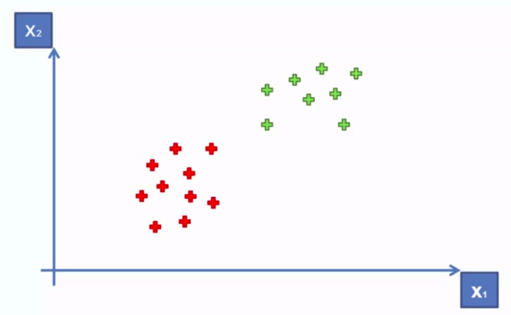
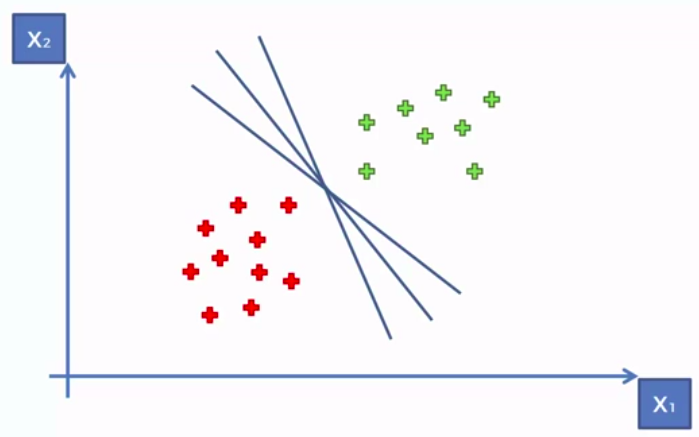
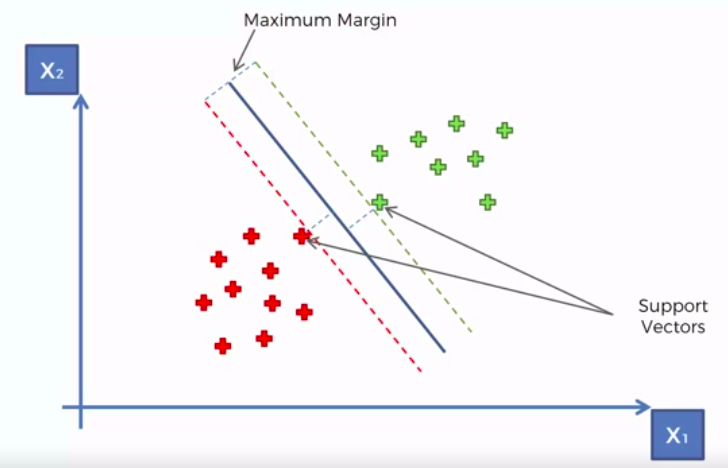
Whats so special about SVM?

Kernel SVM
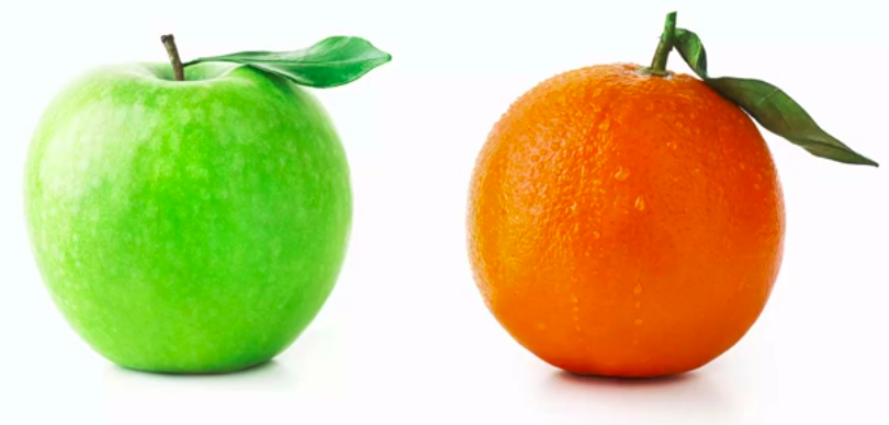
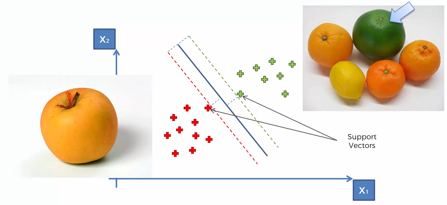
SVM separates well these points

What about these points?

What about these points?
What about these points?
What about these points?
What about these points?
What about these points?
?
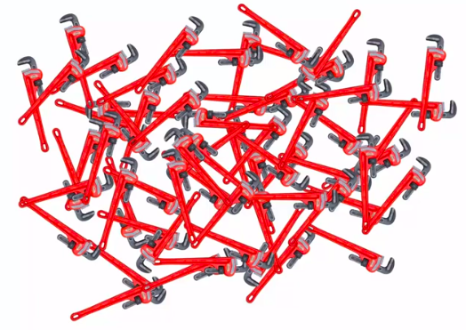
Because the data points are not LINEARLY SEPARABLE

A Higher Dimensional Space
Mapping to a higher dimension 1D Space

Move everythig to the left by (x-5)


Mapping to a higher dimension 2D Space


Mapping to Higher Dimensional Space can be highly compute-intensive
The Kernel Trick
The Gaussian RBF Kernel


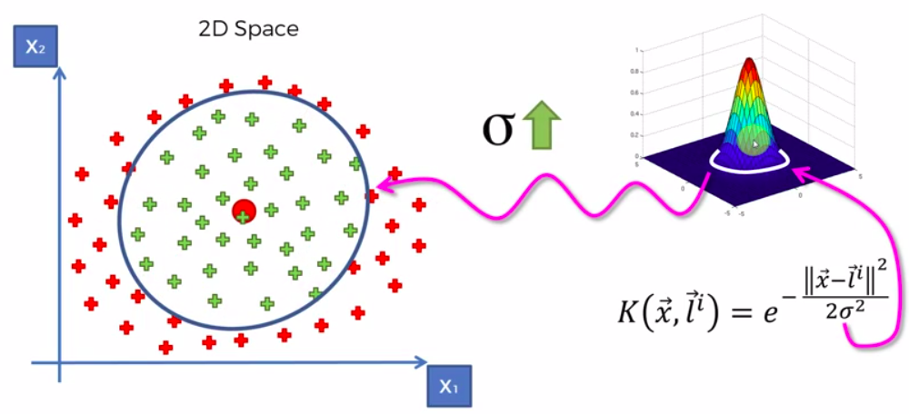


Types of Kernel Functions

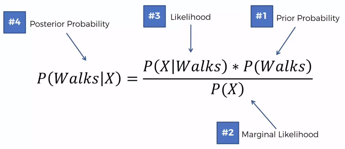
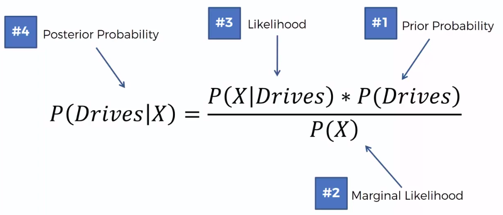
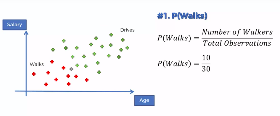
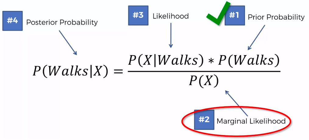
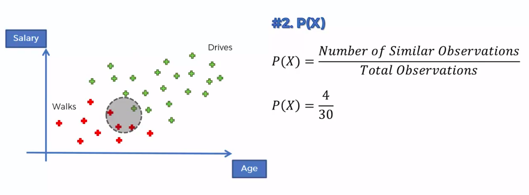
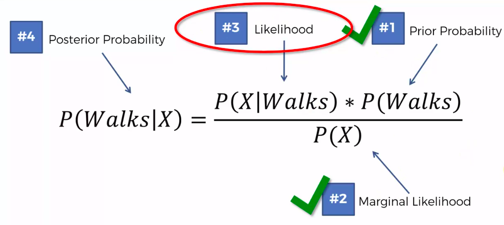
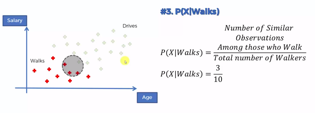
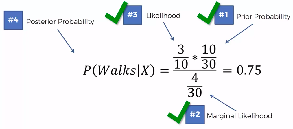
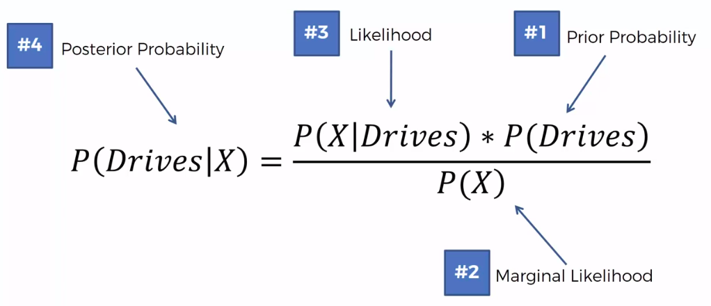
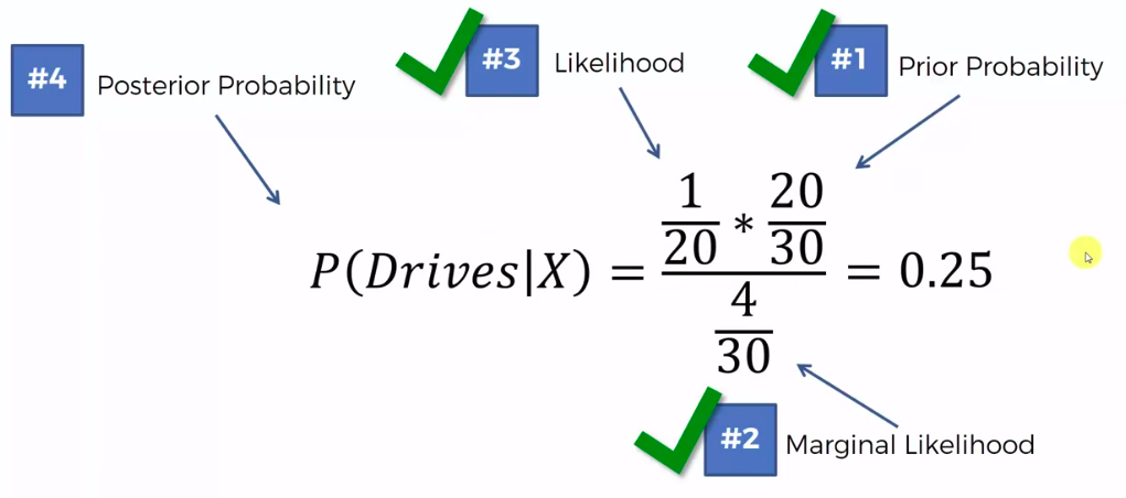
Naive Bayes
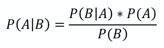
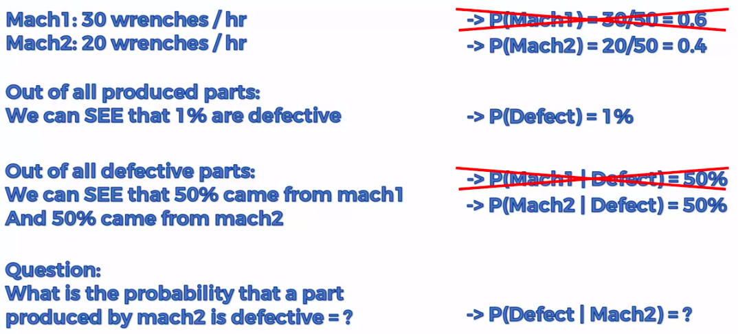
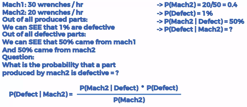
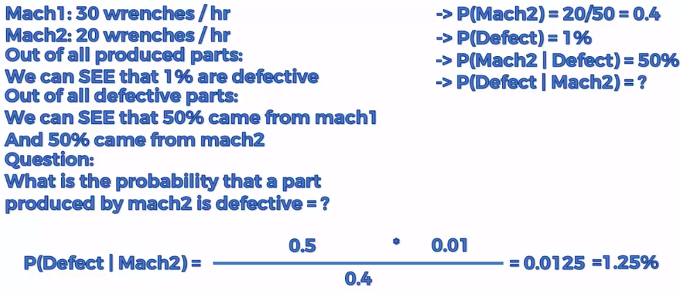
Bayes Theorem
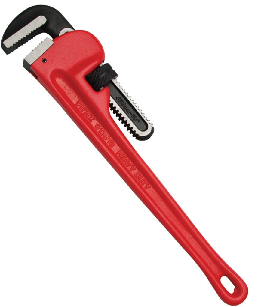
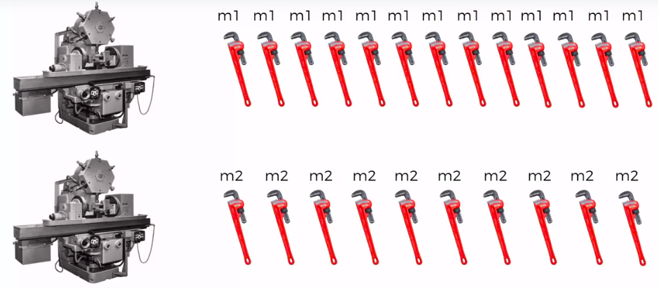
Defective Wrenche
What's the probability?
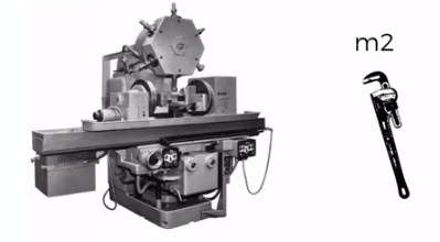
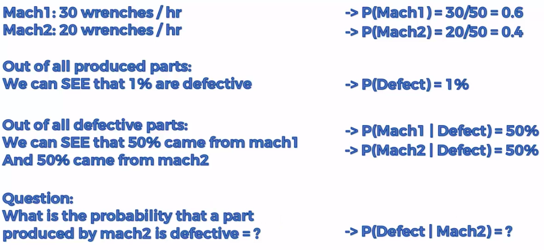
Mach1: 30 wrenches/hr
Mach2: 20 wrenches/hr
Out of all produced parts:
We can SEE that 1% are defective
Out of all defective parts:
We can SEE that 50% came from mach1 And 50% cam from mach2
Question:
What is the probability that a part produced by mach2 is defective = ?

Plan of Attack
Step 1
Step 2
Step 3
Assign class based on probability
Ready ?
Step 1
Step 1
Step 1
Step 1
Step 1
Step 1
Step 2
Step 2
Step 3
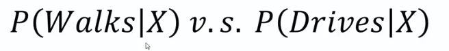
0.75 VS 0.25
0.75 > 0.25
Q: Why "Naive"?
A: Independence Assumption
Q: More than 2 features/classes?
Decision Tree
CART
Classification And Regression Trees
Classification Trees
Regression
Trees
Random Forest Classification
Ensemble Learning
Random Forest
STEP 1: Pick at random K data points from the Training set.
STEP 2: Build the tree associated to these K data points.
STEP 3: Choose the number Ntree of trees we want to build and repeat STEPS1 & 2
STEP 4: For a new data point, make each one of your Ntree trees predict value of Y to for the data point in question, and assign the new data point the average across all of the predicted Y values.

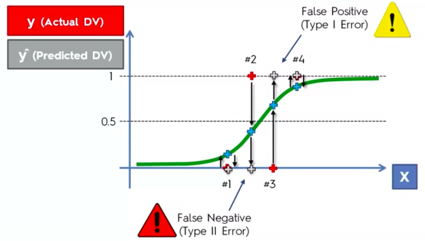
Evaluating Classifier Model Performance
False Positives
&
False Negatives
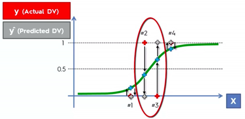
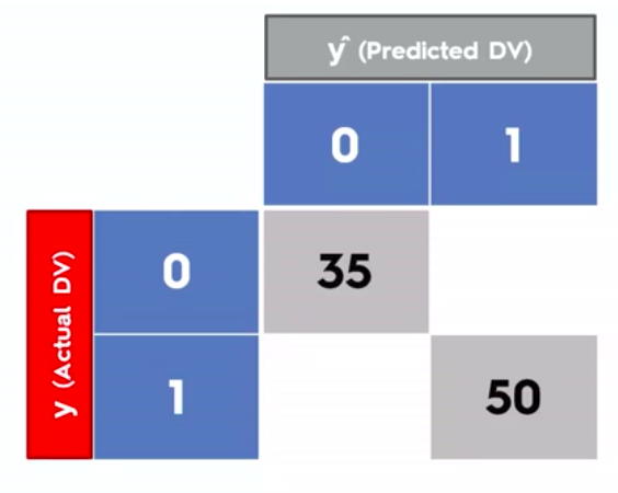
Confusion Matrix
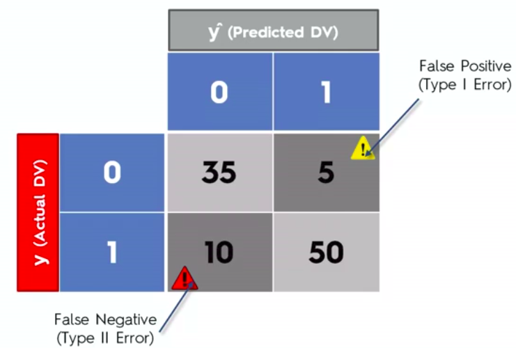
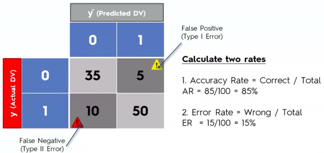
Accuracy Paradox


Pros and the Cons of each classification model

-
If our problem is linear, we should go for Logistic Regression or SVM.
-
If our problem is non linear, we should go for K-NN, Naive Bayes, Decision Tree or Random Forest.
- Logistic Regression or Naive Bayes when we want to rank our predictions by their probability. For example if we want to rank our customers from the highest probability that they buy a certain product, to the lowest probability. Eventually that allows us to target our marketing campaigns. And of course for this type of business problem, we should use Logistic Regression if our problem is linear, and Naive Bayes if our problem is non linear.
- SVM when we want to predict to which segment our customers belong to. Segments can be any kind of segments, for example some market segments we identified earlier with clustering.
- Decision Tree when we want to have clear interpretation of our model results,
- Random Forest when we are just looking for high performance with less need for interpretation.
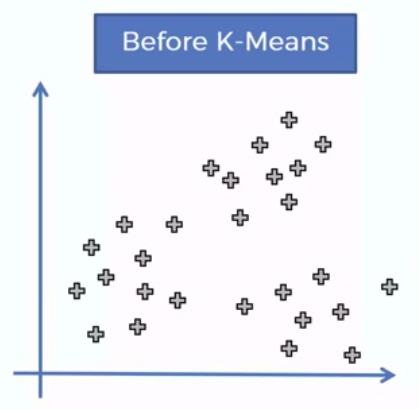
Clustering
Clustering is similar to classification, but the basis is different. In Clustering we don’t know what we are looking for, and we are trying to identify some segments or clusters in our data. When we use clustering algorithms on our dataset, unexpected things can suddenly pop up like structures, clusters and groupings we would have never thought of otherwise.
K-Means Clustering
We can apply K-Means for different purposes:
- Market Segmentation,
- Medicine with for example tumor detection,
- Fraud detection
- to simply identify some clusters of your customers in your company or business.
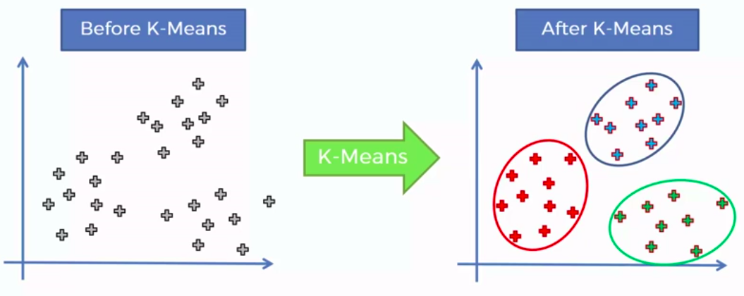
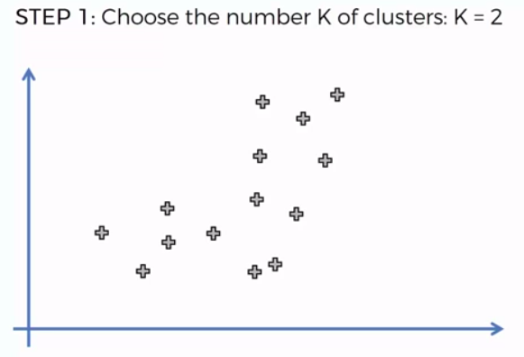
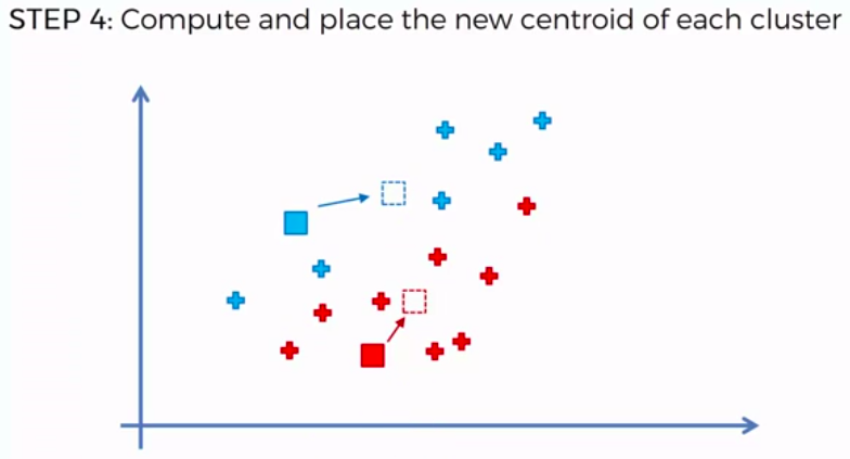
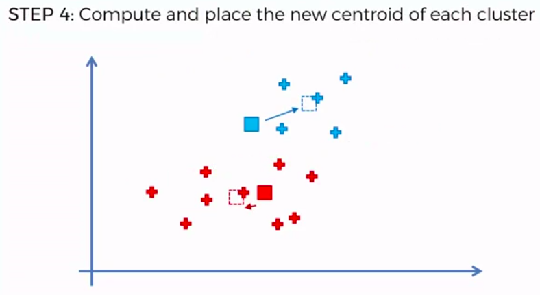
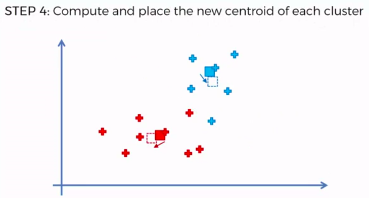
How did K-Mean did it?
STEP 1: Choose the number of K clusters
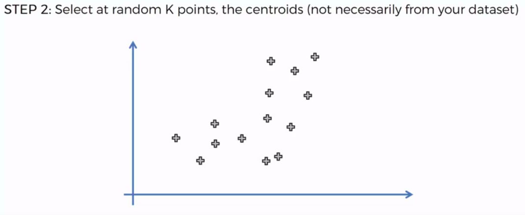
STEP 2: Select at random K points, the centroids (not necessarily from our dataset)
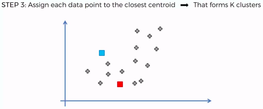
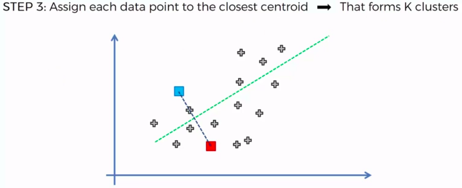
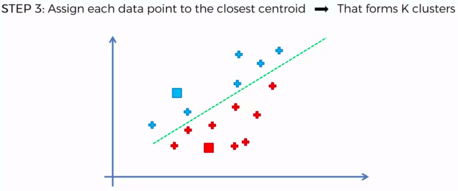
STEP 3: Assign each data point to the closest centroid -> that forms K clusters
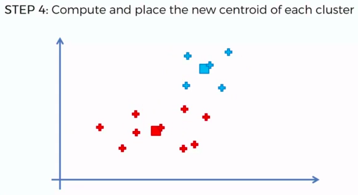
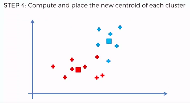
STEP 4: Compute and place the new centroid of each cluster
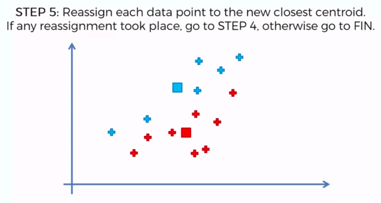
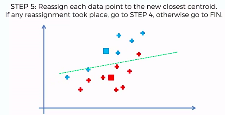
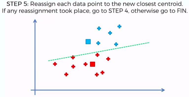
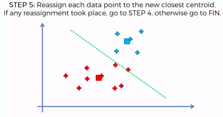
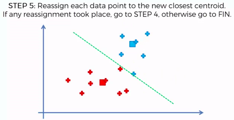
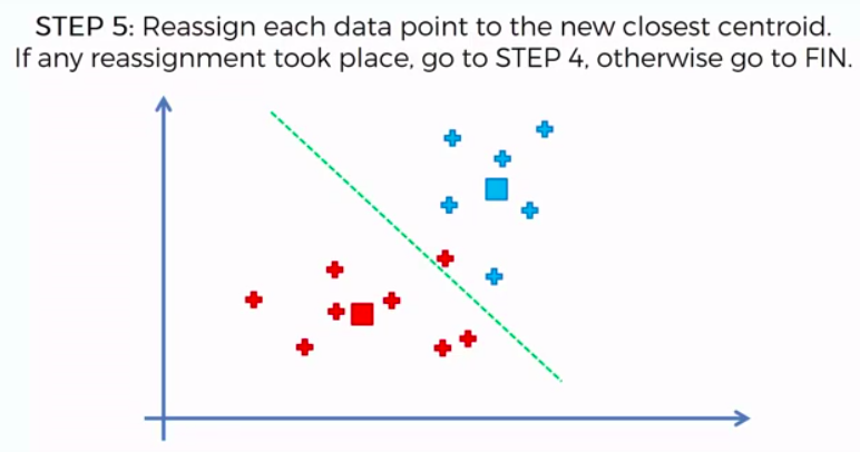
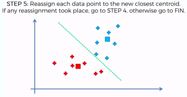
STEP 5: Reassign each data point to the new closest centroid. If any reassignment took place, go to Step 4. Otherwise go to FIN.
FIN: Our Model is Ready


K-Means Random Initialization Trap


What would happen if we had a bad random initialization?


Choosing the right number of clusters


A few minutes ago...


Hierarchical Clustering

2 Approach
Agglomerative
&
Divisive
Agglomerative HC
STEP 1: Make each data point a single-point cluster -> That forms N clusters
STEP 2: Take the two closest data points and make them one cluster -> That forms N-1 clusters
STEP 3: Take the two closest clusters and make them one cluster -> That forms N-2 clusters
STEP 4: Repeat STEP 3 until there is only one cluster
FIN: Our Model is Ready

Distance Between Clusters


Lets Begin !


Dendogram
How does it work?


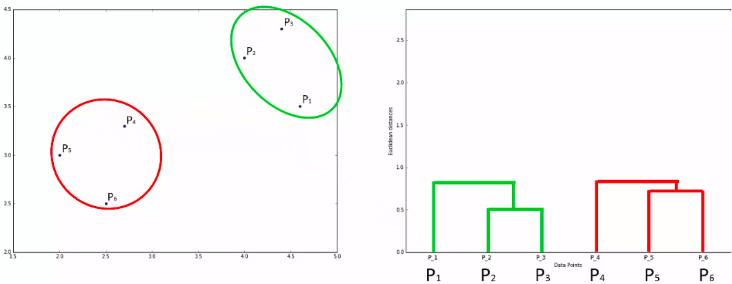

Dendogram
How do we use it?


Another Example:

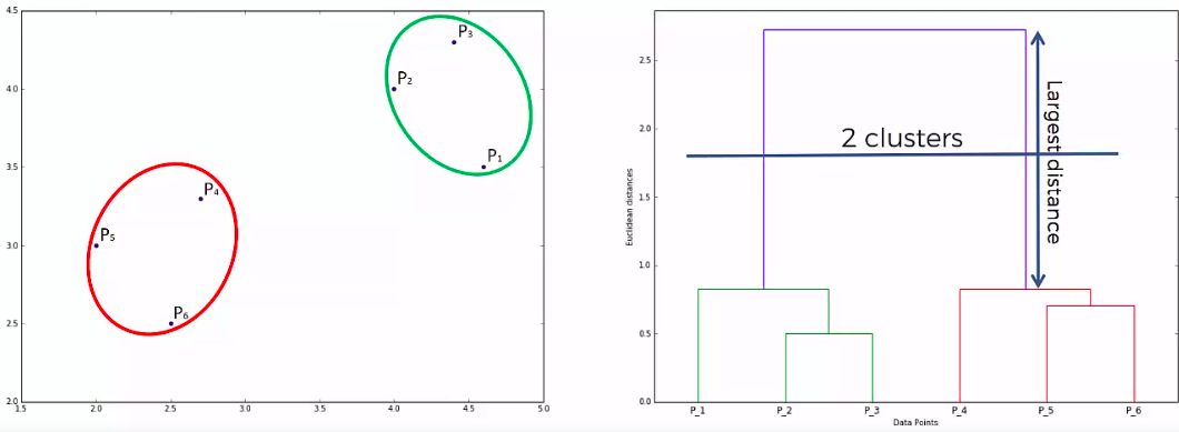
Dendogram
get optimal number of clusters

Quiz :)


Clustering
Pros and Cons

Association Rule Learning
(Apriori)

People who bought also bought ...
ARL:
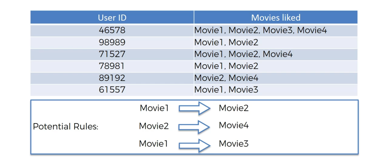
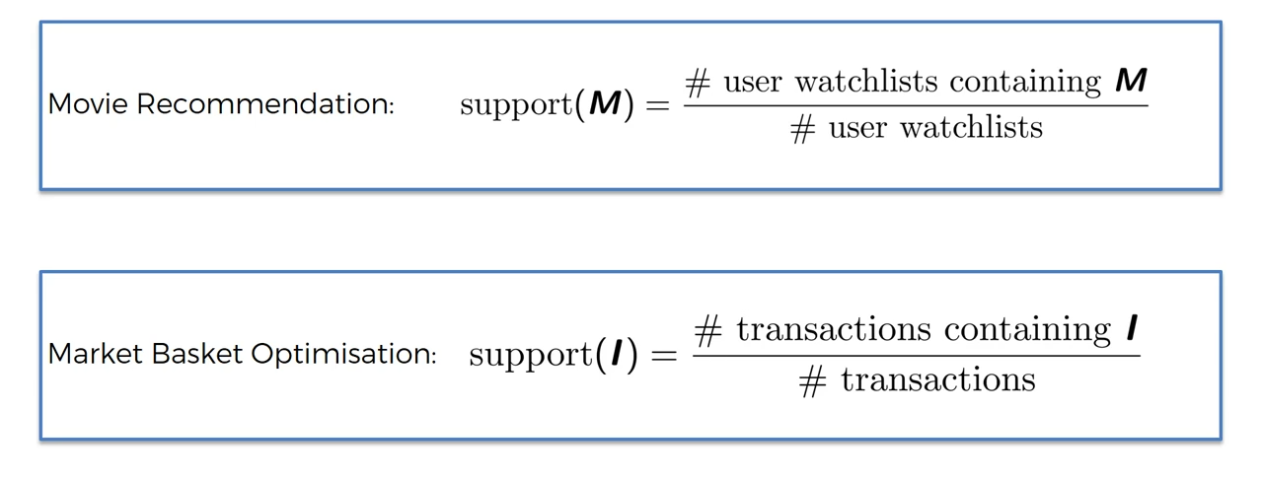
Movie Recommendation
ARL:
Market Basket Optimisation

Step 1:
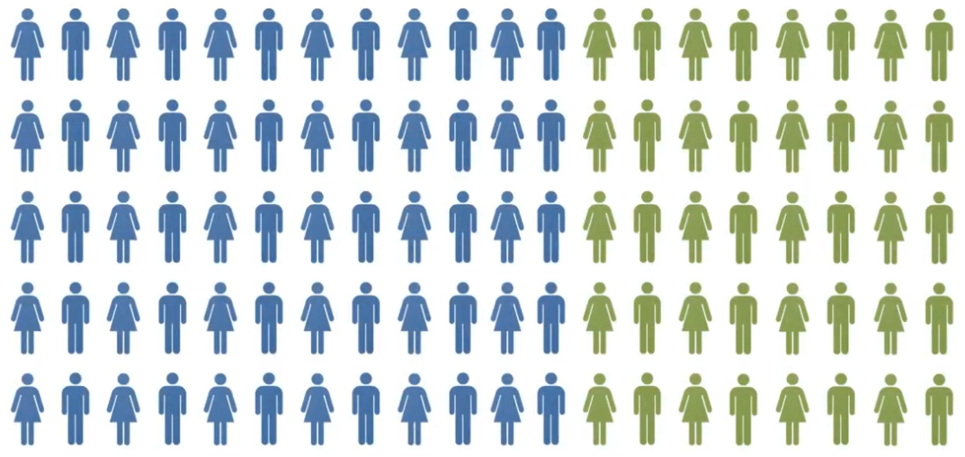
Find Support
Apriori - Support
Apriori - Support
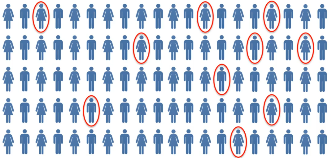
Apriori - Support
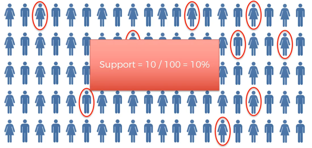
Apriori - Support
Step 2:
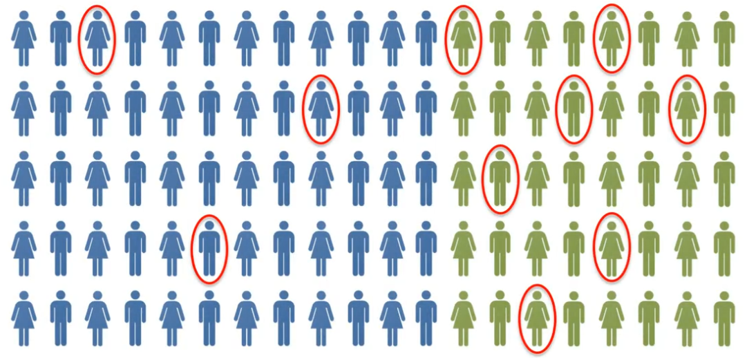
Find Confidence
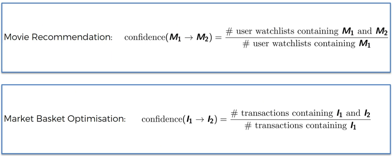
Apriori - Confidence
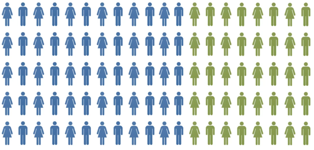
Apriori - Confidence

Apriori - Confidence
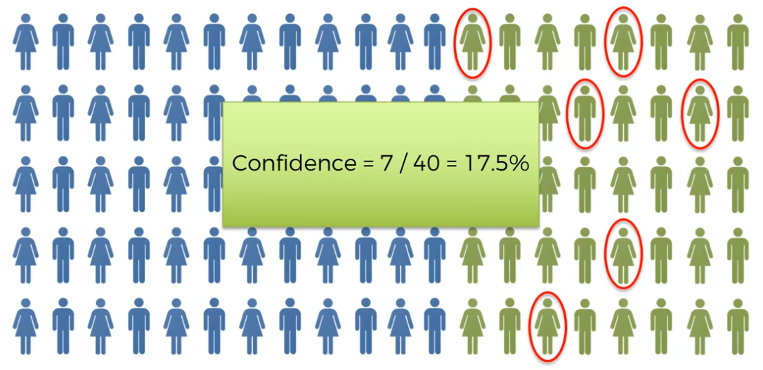
Apriori - Confidence
Step 3:
Calculate Lift
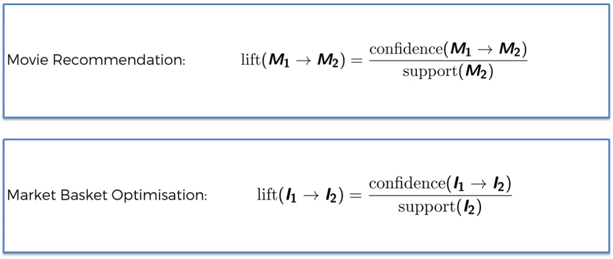
Apriori - Lift
Apriori - Lift
Apriori - Lift
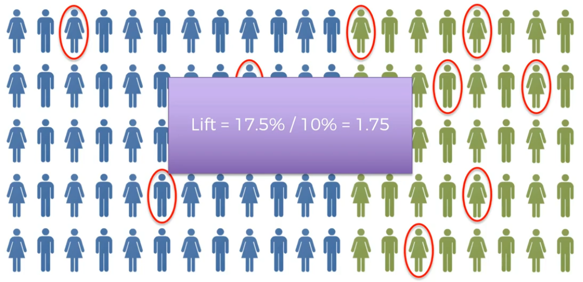
Apriori - Lift
Apriori Algorithm
STEP 1: Set a minimum support and confidence
STEP 2: Take all the subsets in transactions having higher support than minimum support
STEP 3: Take all the rules of these subsets having higher confidence than minimum confidence
STEP 4: Sort the rules by decreasing lift
Association Rule Learning
(Eclat)
People who bought also bought ...
ARL:
Movie Recommendation
ARL:
Market Basket Optimisation
Eclat - Support
Eclat Algorithm
STEP 1: Set a minimum support
STEP 2: Take all the subsets in transactions having higher support than minimum support
STEP 3: Sort these subsets by decreasing support
Reinforcement Learning
(Online Learning)
[UCB]
Reinforcement learning has been one of the most researched machine learning algorithms. As an algorithm that can be closely related to how human beings and animals learn to interact with the environment, reinforcement learning has always been given huge importance especially when it comes to branches of Artificial Intelligence such as robotics
Used to solve interacting problems where the data observed up to time t is considered to decide which action to take at time t + 1. It is also used for Artificial Intelligence when training machines to perform tasks such as walking. Desired outcomes provide the AI with reward, undesired with punishment. Machines learn through trial and error.

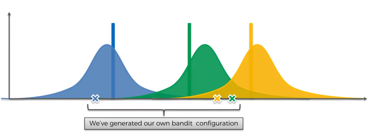
The Multi-Armed Bandit Problem


Example used for training purpose. No affiliation with coca-cola
Upper Confidence Bound (UCB)
The Multi-Armed Bandit Problem
- We have d arms. For example, arms are ads that we display to users each time they connect to a web page.
- Each time users connect to we web page, that make a round
- At each round n, we chose one ad to display to the user.
- At each round n, ad i gives reward if the user clicked on the ad i, 0 if the user didn't
- Our goal is to maximize the total reward we get over many rounds.

Upper Confidence Bound Algorithm


Reinforcement Learning
(Online Learning)
[Thompson Sampling]
Reinforcement learning has been one of the most researched machine learning algorithms. As an algorithm that can be closely related to how human beings and animals learn to interact with the environment, reinforcement learning has always been given huge importance especially when it comes to branches of Artificial Intelligence such as robotics
The Multi-Armed Bandit Problem
The Multi-Armed Bandit Problem
- We have d arms. For example, arms are ads that we display to users each time they connect to a web page.
- Each time users connect to we web page, that make a round
- At each round n, we chose one ad to display to the user.
- At each round n, ad i gives reward if the user clicked on the ad i, 0 if the user didn't
- Our goal is to maximize the total reward we get over many rounds.
Bayesian Inference

Thompson Sampling Algorithm


And so on...

UCB
vs
THOMPSON SAMPLING

Natural Language Processing
Natural-language processing (NLP) is an area of computer science and artificial intelligence concerned with the interactions between computers and human (natural) languages. NLP is used to apply Machine Learning models to text and language.
Example use:
Teach machines to understand what is said in spoken and written word is the focus of NLP. Whenever we dictate something into our iPhone/Android device that is then converted to text,that's an NLP algorithm in action
The history of natural language processing generally started in the 1950s, although work can be found from earlier periods. In 1950, Alan Turing published an article titled "Intelligence" which proposed what is now called the Turing test as a criterion of intelligence
Up to the 1980s, most natural language processing systems were based on complex sets of hand-written rules. Starting in the late 1980s, however, there was a revolution in natural language processing with the introduction of machine learning algorithms for language processing
source: wiki
NLP Uses
- Sentiment analysis. Identifying the mood or subjective opinions within large amounts of text, including average sentiment and opinion mining.
- Use it to predict the genre of the book
- Question Answering (Chat Bot)
- Use NLP to build a machine translator or a speech recognition system
- Document Summarization
Some of Main NLP Libraries
- Natural Language Toolkit - NLTK == TM
- SpaCy
- Stanford NLP
- OpenNlp
NLTK - Part of Speech (PoS)

NN = Noun
JJ = Adjective
DT = Determiner
CD = Cardinal/Number
Semantic Information
Words & Relationship

NLP: Bag of Words
A very popular NLP Model - It is a model used to preprocess the texts to classify before fitting the classification algorithms on the observations containing the texts.
It involve 2 things:
- A vocabulary of known words
- A measure of the presence known words
Deep Learning

Storage Evolution
5MB
10MB
256MB


What is Deep Learning

Geoffrey Hinton
- Did research in Deep Learning in 1980's
- Works at google
- "Otai" Deep Learning
We trying to mimic how human brain operate.

Human Brain has approx 100B neurons and each neuron is connected to as many as about thousand of its neighbour
Neuron View in Microscope
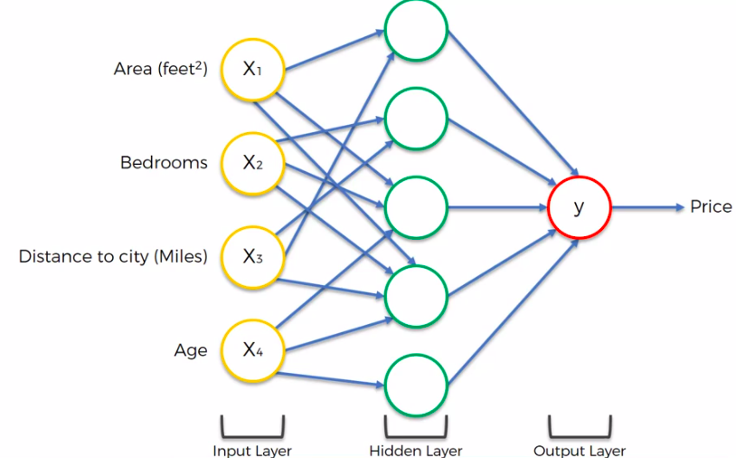
Artificial Neural Network


There is nothing deep here...
But why does it called deep learning?
Because it has alot and alot and alot of hidden layers and we connect everything


Artificial Neural Network
We will learn:
- The neuron
- The activation function
- How do neural network work
- How do neural network learn
- Gradient Descent
- Stochastic Gradient Descent
- Backpropagation
The Neuron


The Neuron


Output Value


Synapse - weight

What happen in Neuron?

Neuron - Step 1
Sum all the input values it get

Neuron - Step 2
Apply activation function

Neuron - Step 3
Pass the signal to the next signal/neuron
The Activation Function

Threshold Function

Sigmoid Function

Rectifier

Hyperbolic Tangent (tanh)
Quick Exercise
Q: Assuming the DV is binary (y=0 or y=1) which threshold function would you use?


How do NNs work?


The Power of Hidden Layer


How do NNs learn?

Single Layer Feed Forward


Something that can learn and adjust itself
Perceptron algorithm was invented in 1957 at the Cornell Aeronautical Laboratory by Frank Rosenblatt

Cost Function: What is the error we have in our prediction. Our goal is to minimize the error. The lower the cost function the closer y-hat to y

Feed information back to NN. Our goal is to minimize the cost function, all we can do is update the weight
FYI, for now we only deal with 1 row


Feed this values into NN

Everything get adjusted, weight get adjusted

Feed this row again

Everytime y-hat is changing our cross function also change


Usually we wont get cross function = 0. But this is for demo purposes
Up until now,
we just dealing with 1 row
Let's see what happen when we have multiple rows

In reality, there is only 1 NN for multiple rows. I split it up for understanding purpose
The goal here is to minimize the cost function. As soon as we found the minimum CS, that means that is our final NN (weight has been adjusted): we have found the optimal weight
This whole process is called backpropagation
Gradient Descent
How the weights are adjusted

Brute force approach:
Test lot of possible weight
If we have 1 weight to optimize, this might work.
But as we increase number of weight/synapse in our network we have to face ...
Curse Of Dimensionality
Remember the prev example?
Where we Run NN for property evaluation
This is what its looked like after it was trained up already
This is the actual NN before it was trained or before we know what are the weights

How could we brute force our weight through a NN of this size


Gradient Descent
Faster way to find the best option
Lets start..
- Look at our angle of cross function
- Find out if the slope +ve or -ve (if -ve -> downhill)
- To the right is downhill, to the left is uphill


In simple term, that's how we find the best weight. Of course its not going to be like a ball rolling. It's going to be zig-zag type of approach. But, its easier and more fun to remember it this way.

Example: Gradient Descent (2D)

Example: Gradient Descent (3D)

Stochastic Gradient Descent
Gradient Descent require cost function to be convex. What if our function is not convex?


What if our cost function is not convex?
That could happen if we choose cost function which is not the squared diff between y-hat and y. Or if we do choose CS like that but then in multi dimension space it can turn to something that is not convex
Sthocastic Gradient Descent doesnt require CS to be convex
Batch Gradient Descent

Sthocastic Gradient Descent

Sthocastic Gradient Descent

Sthocastic Gradient Descent

So, basically we adjusting the weight after a single row rather than doing everything together


Sthocastic gradient descent is faster. Its doing every single row 1 at a time, it doesn't have to load up all the data into memory and wait until all those rows run together
Backpropagation


Backpropagation allow us to adjust the weight all of them at the same time
Training the ANN with Stochastic Gradient Descent
STEP 1: Randomly initialize the weights to small numbers close to 0 (but not 0)
STEP 2: Input the observation of our dataset in the input layer, each feature in one input node
STEP 3: Forward-Propagation: from left to right, the neurons are activated in a way that the impact of each neuron's activation is limited by the weights. Propagate the activations until getting the predicted result y
Training the ANN with Stochastic Gradient Descent
STEP 4: Compare the predicted result to the actual result. Measure the generated error
STEP 5: Back-Propagation: from right to left, the error is back-propagated. Update the weights according to how much they are responsible for the error. The learning rate decides by how much we update the weights.
Training the ANN with Stochastic Gradient Descent
STEP 6: repeat Steps 1 to 5 and update the weights after each observation (reinforcement Learning). Or: Repeat Steps 1 to 5 but update the weights only after a batch of observations (Batch Learning).
STEP 7: When the whole training set passed through the ANN, that makes an epoch. Redo more epochs.
Principal Component Analysis
(PCA)
- Noise Filtering
- Visualization
- Feature Extraction
- Stock Market Predictions
- Gene data analysis
PCA Goals
- Identify patterns in data
- Detect the correlation between variables
- Reduce the dimensions of a d-dimensional dataset by projecting it onto a (k)-dimensional subspace where (k<d)

5 Main Step for PCA
Conclusion of PCA
-
Learn about the relationship between X and Y values
-
Find list of principal axes
Before starts with hands on training...

From the m independent variables of our dataset, PCA extracts p <= m new independent variables that explain the most the variance of the dataset,regardless of the dependent variable
The fact that the DV is not considered makes PCA an unsupervised model
Linear Discriminant
Analysis
(LDA)
LDA
- Used as a dimensionality reduction technique
- Used in the pre-processing step for pattern classification
- Has the goal to project a dataset onto a lower-dimensional space
Hurmmm..
Sounds similar to PCA right?
LDA differs because in addition to finding the component axises with LDA, we are interested in the axes that maximize the separation between multiple classes
Breaking it down further...
The goal of LDA is to project feature space (a dataset n-dimensional samples) onto a small subspace k (where k<=n-1) while maintaining the class-discriminatory information.
Both PCA and LDA are linear transformation techniques used for dimensional reduction. PCA is described as unsupervised but LDA is supervised because of the relation to the dependent variable

5 Main Step for LDA

Before starts with hands on training...
LDA in few words...
From the n independent variables of our dataset, LDA extractrs p <= n new independent variables that separate the most the classes of the dependent variable.
The fact that the DV is considered, makes LDA a supervised mode
K-Fold
Cross Validation

Splitting the training set into 10 folds.
k = 10, most of the time k=10

We train our model on 9 folds and we test on last remaining fold


Then, we take an average of the difference accuracy of 10 evaluations and also compute standard deviation to have a look at the variance. Our analysis will be much more relevant

- Lower Left: Good accuracy & Small Variance
- Lower Right: Large Accuracy & High Variance
- Upper Left: Small Accuracy & Low Variance
- Upper Right: Low Accuracy & High Variance
Grid Search
XGBoost
One of the most popular algorithm in ML and a very powerful model especially on large datasets
Gradient boosting is a machine learning technique for regression and classification problems, which produces a prediction model in the form of an ensemble of weak prediction models, typically decision trees.
(Wikipedia definition)
What is Gradient Boosting?
Boosting is an ensemble technique in which the predictors(IV) are not made independently, but sequentially.


Why XGBoost?
- Execution Speed
- Model Performance
There are no secrets to success. It is the result of preparation, hard work, and learning from failure. - Colin Powell
THANK YOU
R - Machine Learning
By Abdullah Fathi
R - Machine Learning
Learn how to create machine learning algorithm in R


