Machine Learning
Abdullah Fathi


Introduction
- Machine learning is a subset of artificial intelligence.
- Focuses mainly on designing systems which allow them to learn and make predictions based on some experience which is data.

Machine learning is becoming widespread among data scientist and is deployed in hundreds of products we use daily. One of the first ML application was spam filter
Applications of ML

Applications of ML

Supervised
VS
Unsupervised
Supervised Learning
Training data feed to the algorithm includes a label (answer)
-
Classification
- Most used supervised learning technique
-
Regressions
- Commonly used in ML field to predict continuous value.
- Predict the value of dependant variable based on a set of independant variables (also called predictors or regressors)
Lists of some fundamental supervised learning algorithms
- Linear Regression
- Logistic Regression
- Neares Neighbours
- Support Vector Machine (SVM)
- Decision trees and Random Forest
- Neural Networks
Unsupervised Learning
Training data is unlabeled.
The system tries to learn without a reference
List of unsupervised learning algorithms
- K-mean
- Hierarchical Cluster Analysis
- Expectation Maximization
- Visualization and dimensionality reduction
- Principal Component Analysis
- Kernel PCA
- Locally-Linear Embedding
- Data PreProcessing
-
Regression
- Simple Linear Regression
- Multiple Linear Regression
- Polynomial Regression
- Support Vector Regression (SVR)
- Decision Tree Regression
- Random Forest Regression
- Evaluating Regression Model Performance
-
Classification
- Logistic Regression
- K-Nearest Neighbour (KNN)
- Support Vector Machine (SVM)
- Kernel SVM
- Naive Bayes
- Decision Tree Classification
- Random Forest Classification
- Evaluating Classification Models Performance
-
Clustering
- K-Means Clustering
- Hierarchical Clustering
- Natural Language Processing (NLP)
-
Deep Learning
- Artificial Neural Network
Data Preprocessing
Before begin our journey with machine learning, we need to prepare our data
Regression
Regression models (both linear and non-linear) are used for predicting a real value, like salary for example. If our independent variable is time, then we are forecasting future values, otherwise our model is predicting present but unknown values. Regression technique vary from Linear Regression to SVR and Random Forests Regression
ML Regression Models
- Simple Linear Regression
- Multiple Linear Regression
- Polynomial Regression
- Support Vector for Regression (SVR)
- Decision Tree Classification
- Random Forest Classification
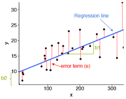
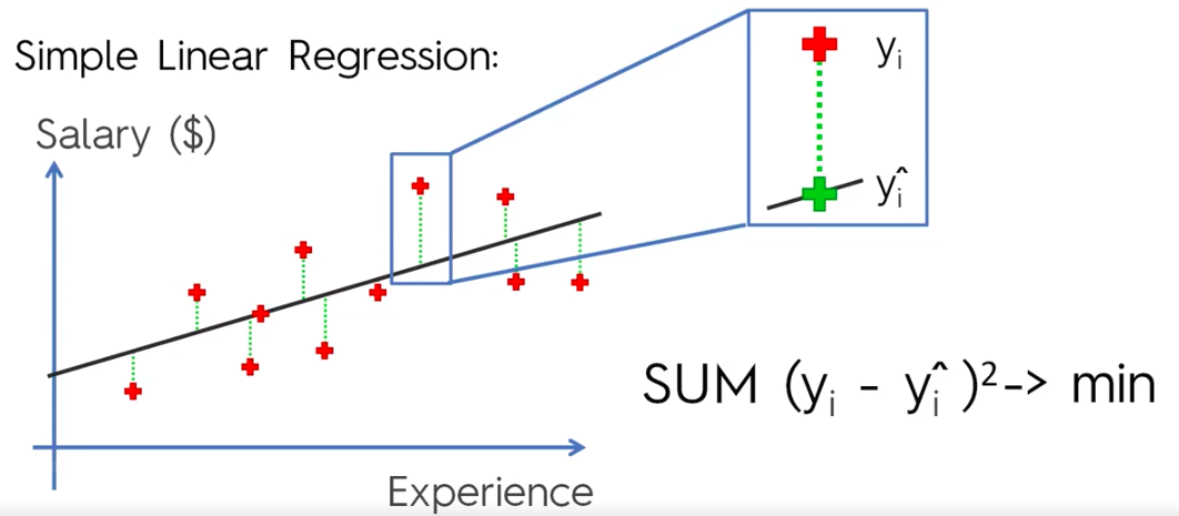
Simple Linear Regression

Simple Linear Regression
y = Dependant Variable (DV)
X = Independant Variable (IV)
b1 = Coefficient
b0 = Constant
lm(formula, data)

# Where
#    formula = A symbolic description of the model to be fitted
#    data = An optional data frame
Multiple Linear Regression

Assumptions of a Linear Regression
- Linearity
- Homoscedasticity
- Multivariate Normality
- Independence of Errors
- Lack of Multicollinearity

Building a Model
Building a Model

Building a Model
5 methods of building models:
- All-in
- Backward Elimination
- Forward Selection
- Bidirectional Elimination
- Score Comparison
Stepwise Regression: Backward Elimination, Forward Selection, Bidirectional Elimination
Method 1:
"All-in"
- Prior knowledge; OR
- You have to; OR
- Preparing for Backward Elimination
Method 2:
Backward Elimination
STEP 1: Select a significance level to stay in the model
(ex: Significance Level (SL) = 0.05)
STEP 2: Fit the full model with all possible predictors (independant variable)
STEP 3: Consider the predictor with the highest P-value. If P > Significance Level (SL), go to STEP 4, otherwise go to FIN
STEP 4: Remove the predictor
STEP 5: Fit model without this variable*
FIN: Our Model is Ready
Method 3:
Forward Selection
STEP 1: Select a significance level to enter the model
(ex: SL = 0.05)
STEP 2: Fit all simple regression models y ~ Xn Select the one with the lowest P-value
STEP 3: Keep this variable and fit all possible models with one extra predictor added to the one(s) we already have
STEP 4: Consider the predictor with the lowest P-value.
If P < SL, go to STEP 3, otherwise go to FIN
FIN: Keep the previous model
Method 4:
Bidirectional Elimination
STEP 1: Select a significance level to enter and to stay in the model (ex: SLENTER = 0.05, SLSTAY = 0.05)
STEP 2: Perform the next step of Forward Selection (new variables must have: P < SLENTER to enter)
STEP 3: Perform ALL steps of Backward Elimination (old variables must have P < SLSTAY to stay)
STEP 4: Now new variables can enter and no old variables can exit
FIN: Our Model is Ready
Method 5:
All Possible Models
STEP 1: Select a criterion of goodness of fit
(ex: Akaike criterion)
STEP 2: Construct All Possible Regression Model:
2^n - 1 total combinations
STEP 3: Select the one with the best criterion
FIN: Our Model is Ready
Ex:
10 columns means
1,023 models
Polynomial Linear Regression


b2X1^2 - give parabolic effect to fit our data better
Polynomial Linear Regression is a special case of Multiple Linear Regression
Support Vector Regression (SVR)
- Kernel: The function used to map a lower dimensional data into a higher dimensional data.
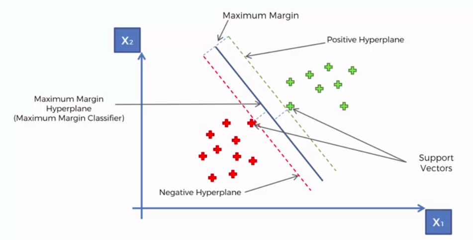
- Hyper Plane: In SVM this is basically the separation line between the data classes. Although in SVR we are going to define it as the line that will will help us predict the continuous value or target value
- Boundary line: In SVM there are two lines other than Hyper Plane which creates a margin . The support vectors can be on the Boundary lines or outside it. This boundary line separates the two classes. In SVR the concept is same.
- Support vectors: This are the data points which are closest to the boundary. The distance of the points is minimum or least.
TERMS
- Support Vector Machines support linear and nonlinear regression that we can refer to as SVR
- Instead of trying to fit the largest possible street between two classes while limiting margins violation, SVR tries to fit as many instances as possible on the street while limiting margins violations.
- The width of the street is controlled by a hyper parameter Epsilon
- SVR performs linear regression in a higher (dimensional space).
- We can think of SVR as if each data point in the training represents it's own dimension. When we evaluate our kernel between a test point and a point in the training set, the resulting value gives us the coordinate of our test point in that dimension.
- The vector we get when we evaluate the test point for all points in the training set, (k vector) is the representation of the test point in the higher dimensional space.
- Once we have that vector, we use it to perform linear regression
Building a SVR
- Collect a training set t = {X, Y}
- Choose a kernel and it's parameters as well as any regularization needed.
- Form the correlation matrix, K
- Train our machine, exactly or approximately, to get contraction coefficients a = {ai}
- Use those coefficients, create our estimator f(X,a,x) = y
Next step is to choose kernel
- Gaussian
Regularization
- Noise
SVR has a different regression goal compared to linear regression. In linear regression we are trying to minimize the error between the prediction and data. In SVR our goal is to make sure that errors do not exceed the threshold

Decision boundary is our Margin of tolerance that is We are going to take only those points who are within this boundary.
Or in simple terms that we are going to take only those those points which have least error rate. Thus giving us a better fitting model.
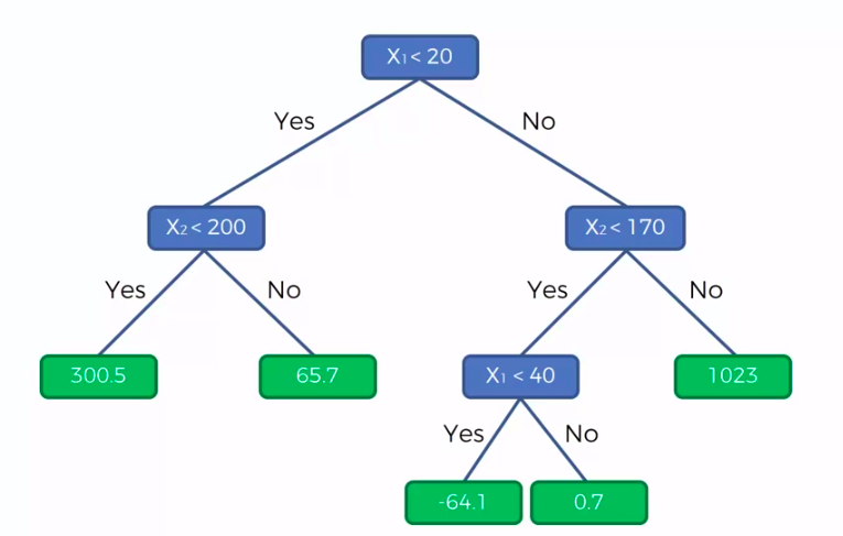
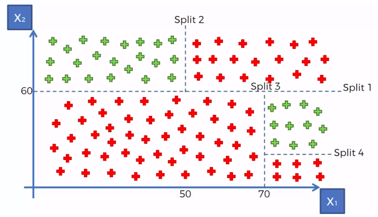
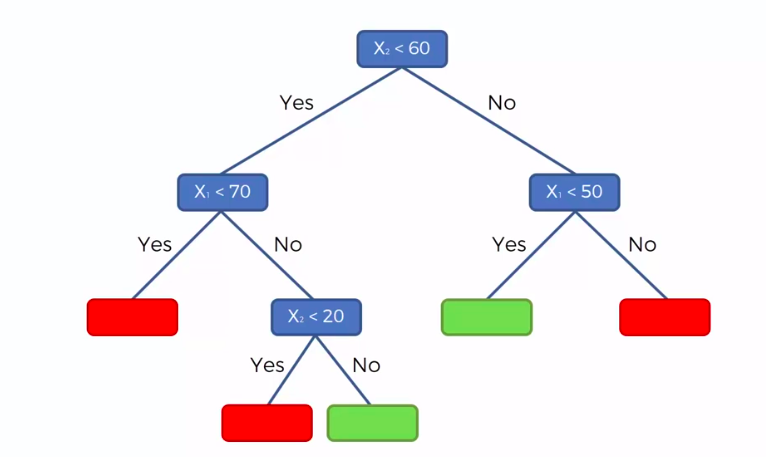
Decision Tree Regression
CART
Classification And Regression Trees
Classification Trees
Regression
Trees
X1 and X2 is Independent Variable
Y is our Dependent Variable which we could not see because it is in another dimension (z-axis)
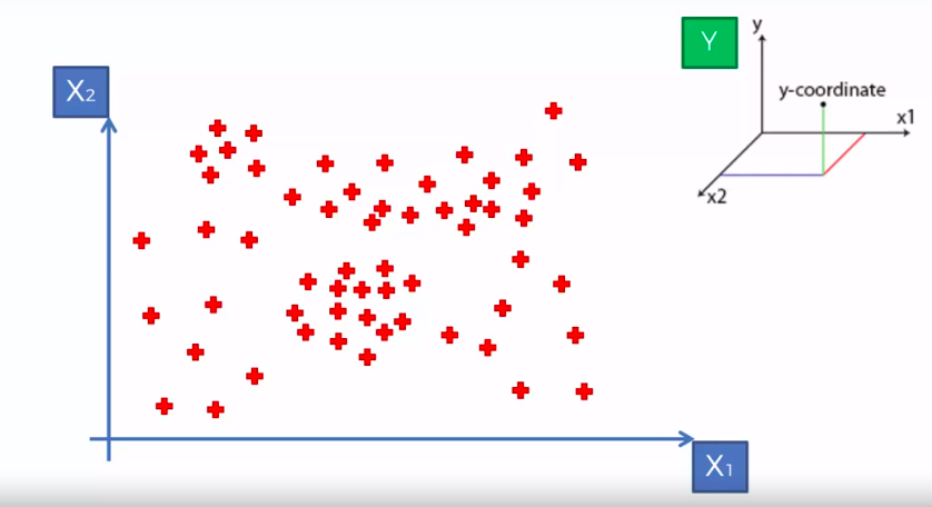
- Scatter plot will be split up into segment
- Split is determine by the algorithm.
- It is actually involve looking at something called information entropy
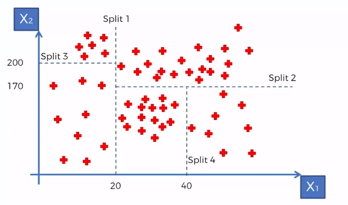
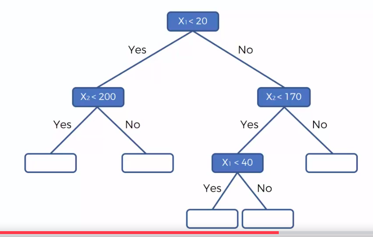
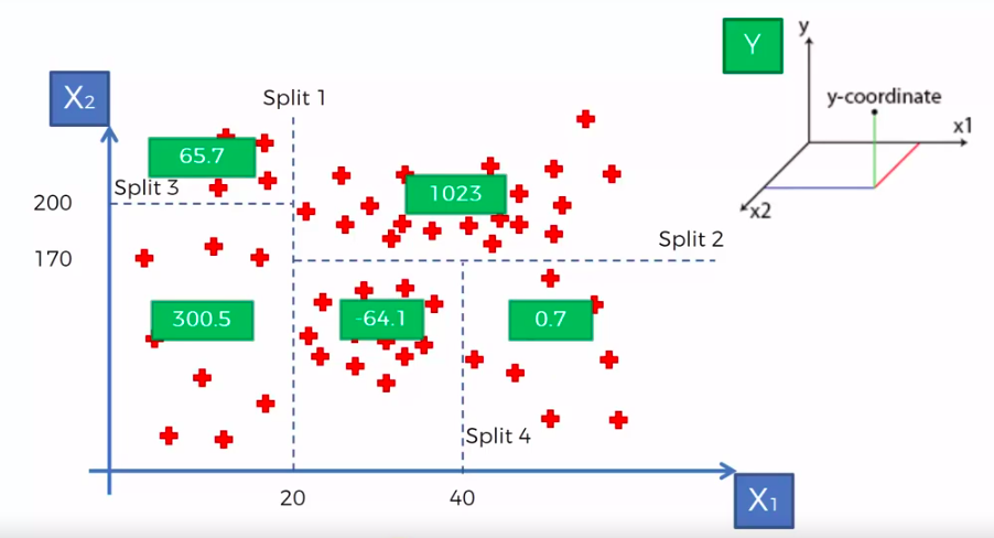
Calculate Mean/Average for each leaf
Random Forest Regression
Random Forest
STEP 1: Pick at random K data points from the Training set.
STEP 2: Build the tree associated to these K data points.
STEP 3: Choose the number Ntree of trees we want to build and repeat STEPS1 & 2
STEP 4: For a new data point, make each one of your Ntree trees predict value of Y to for the data point in question, and assign the new data point the average across all of the predicted Y values.
We are not just predicting based on 1 Tree, We are predicting based on forest of trees. It will improve the accuracy of prediction because we take the average of many prediction
Ensemble training is more stable because one changes of data could really impact one tree, but to impact a forest of trees it would be much harder
Ensemble Training

R-Squared

Adjusted R-Squared


Evaluating Regression Model Performance

Interpreting Linear Regression Coefficients

Pros and the Cons of each regression model

Classification
Unlike regression where we predict a continuous number, we use classification to predict a category. There is a wide variety of classification applications from medicine to marketing. Classification models include linear models like Logistic Regression, SVM, and nonlinear ones like K-NN, Kernel SVM and Random Forests
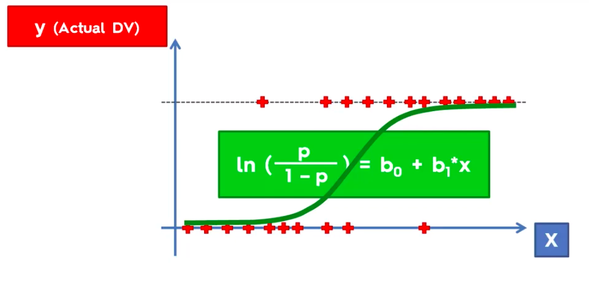
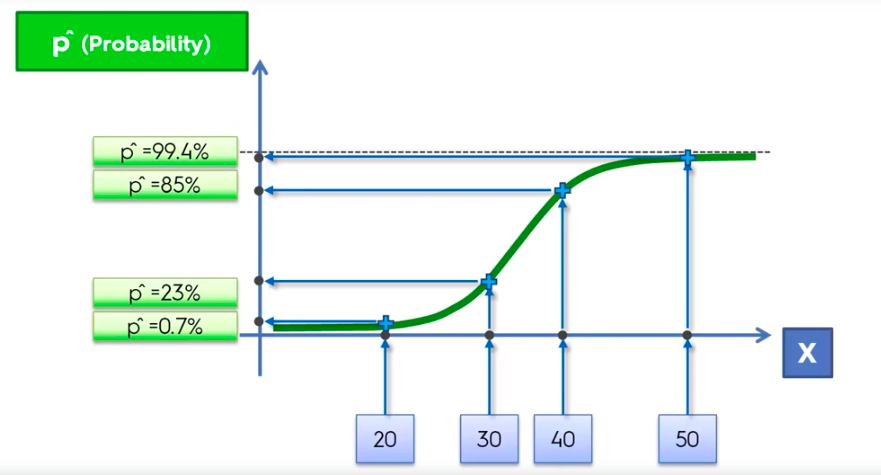
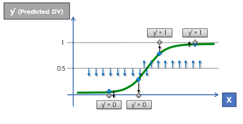
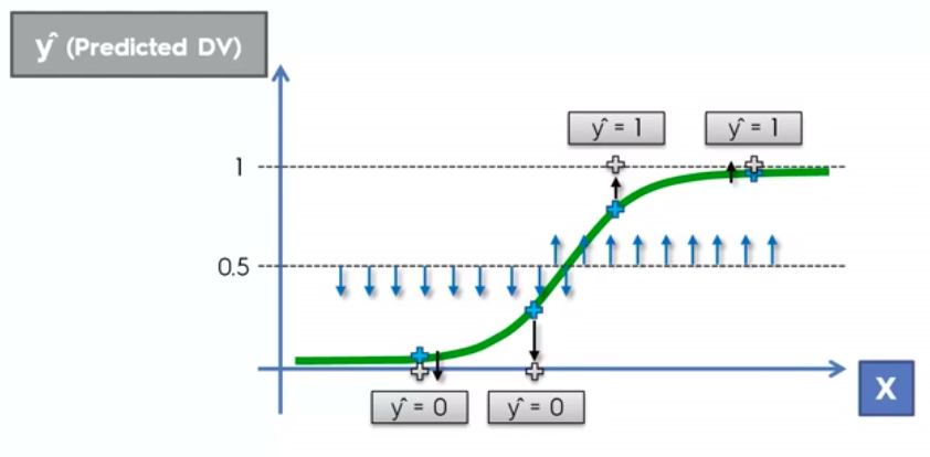
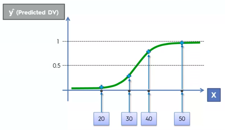
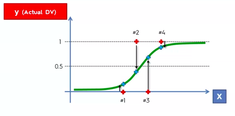
Logistic Regression
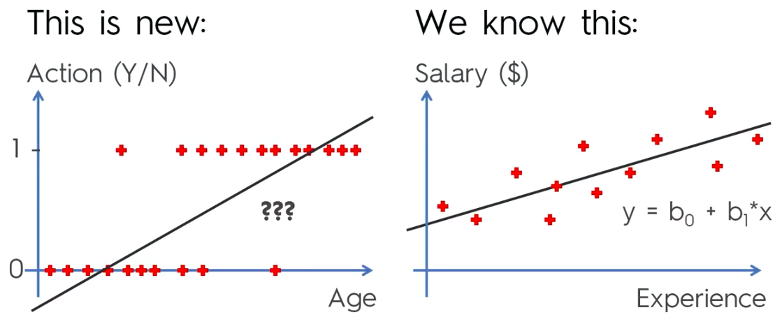
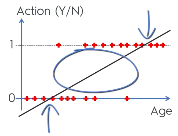
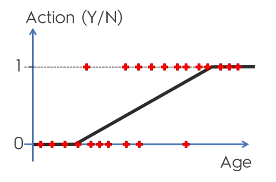
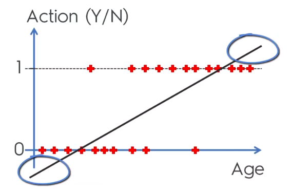
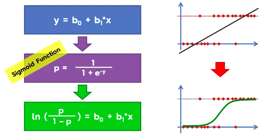
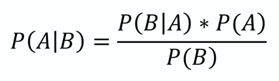
Logistic Regression Equation
library(ElemStatLearn)
set = training_set
X1 = seq(min(set[, 1]) - 1, max(set[, 1]) + 1, by = 0.01)
X2 = seq(min(set[, 2]) - 1, max(set[, 2]) + 1, by = 0.01)
grid_set = expand.grid(X1, X2)
colnames(grid_set) = c('Age', 'EstimatedSalary')
prob_set = predict(classifier, type = 'response', newdata = grid_set)
y_grid = ifelse(prob_set > 0.5, 1, 0)
plot(set[, -3],
     main = 'Logistic Regression (Training set)',
     xlab = 'Age', ylab = 'Estimated Salary',
     xlim = range(X1), ylim = range(X2))
contour(X1, X2, matrix(as.numeric(y_grid), length(X1), length(X2)), add = TRUE)
points(grid_set, pch = '.', col = ifelse(y_grid == 1, 'springgreen3', 'tomato'))
points(set, pch = 21, bg = ifelse(set[, 3] == 1, 'green4', 'red3'))
Visualizing The Results
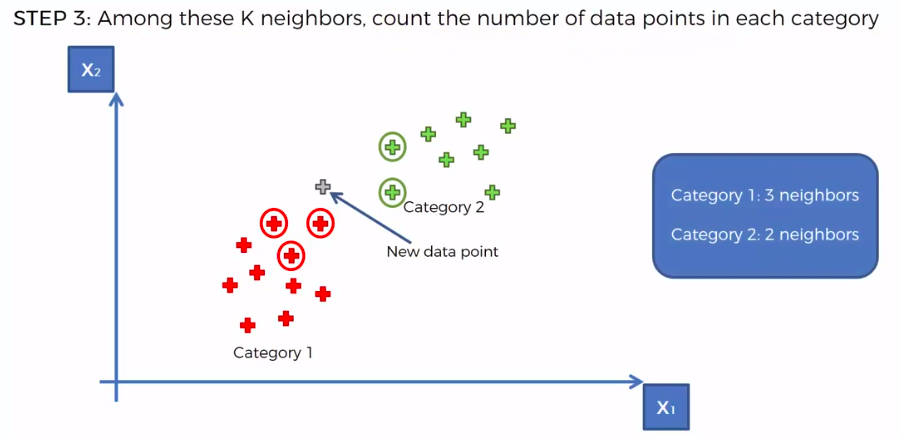
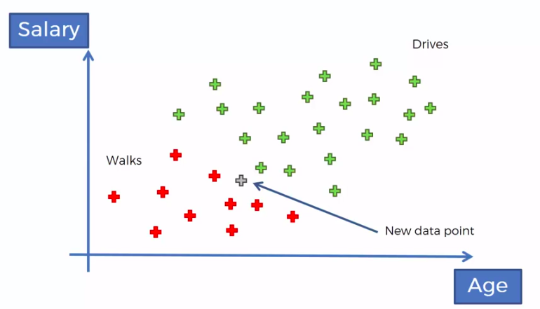
K-Nearest Neighbour
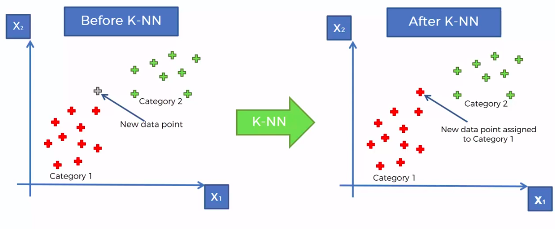
KNN
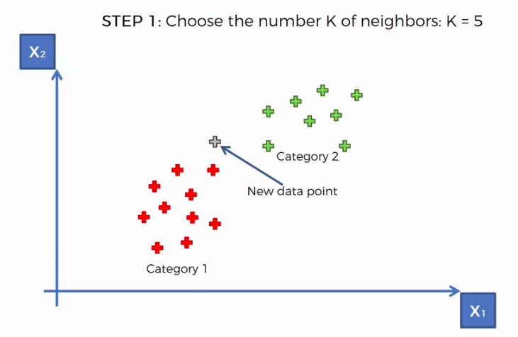
STEP 1: Choose the number K of neighbours
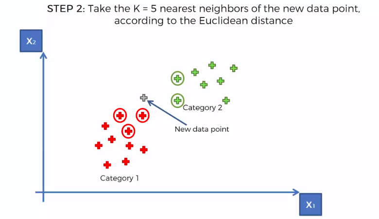
STEP 2: Take the K nearest neighbors of the new data point, according to the Euclidean distance
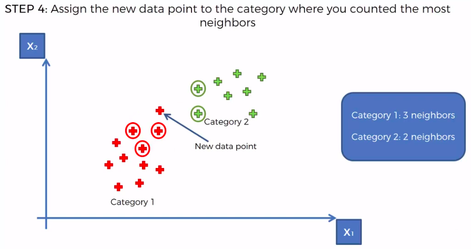
STEP 3: Among these K neighbors, count the number of data points in each category
STEP 4: Assign the new data point to the category where you counted the most neighbours
FIN: Our Model is Ready
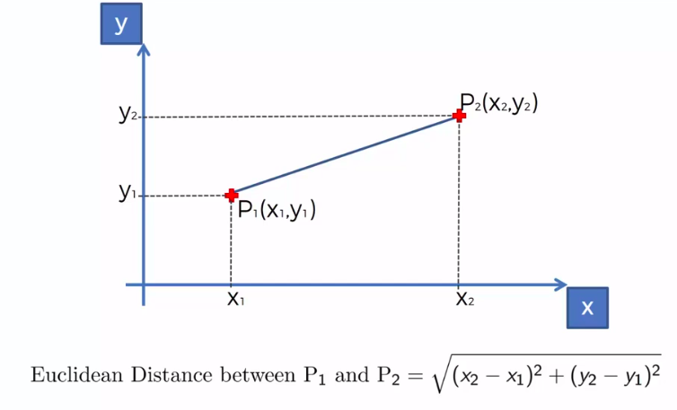
We can use other Distance as well such as Manhattan Distance. But Euclidean is the commonly used for geometry
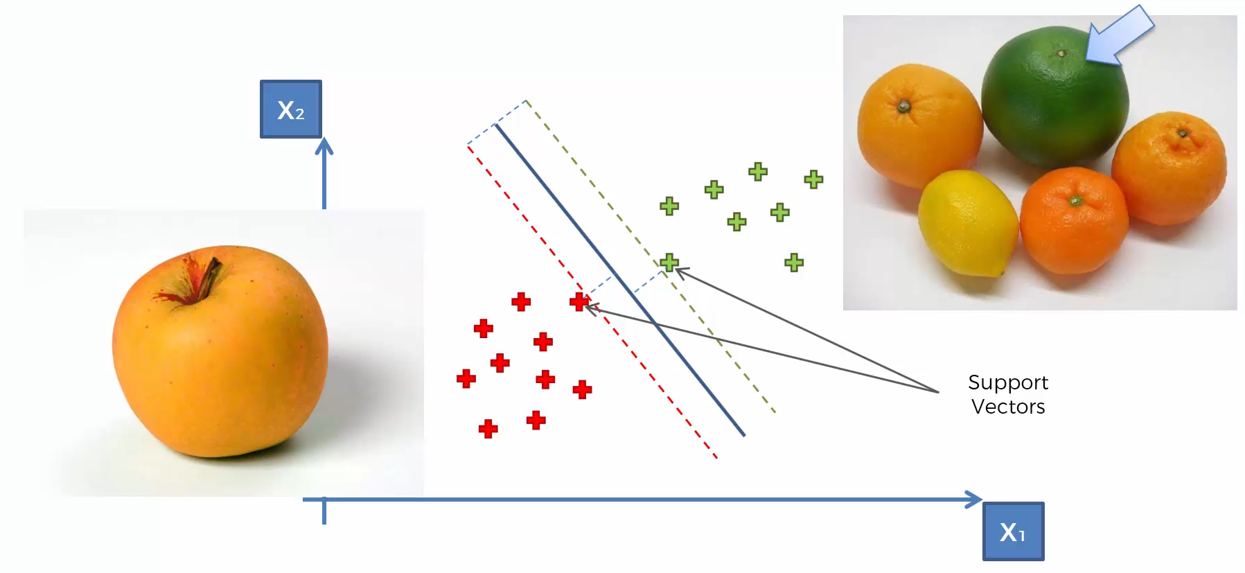
Support Vector Machine (SVM)
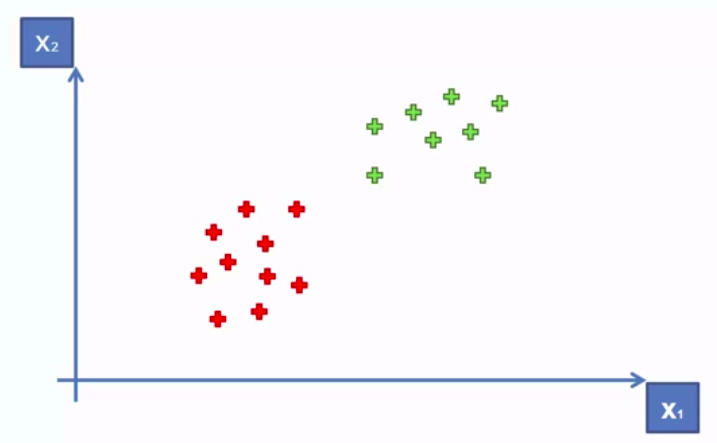
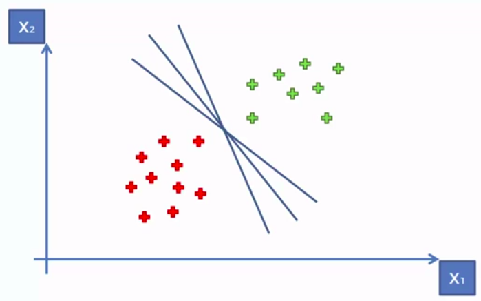
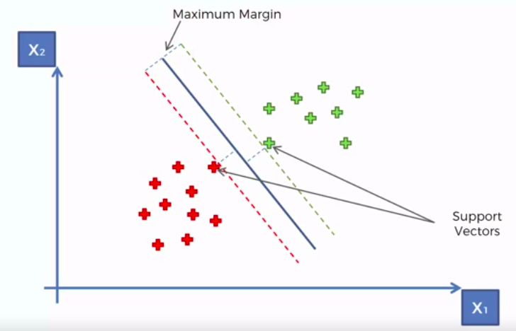
Whats so special about SVM?


Kernel SVM
SVM separates well these points

What about these points?

What about these points?
What about these points?
What about these points?
What about these points?
What about these points?
?
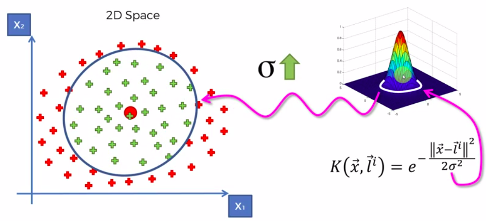
Because the data points are not LINEARLY SEPARABLE

A Higher Dimensional Space
Mapping to a higher dimension 1D Space

Move everythig to the left by (x-5)


Mapping to a higher dimension 2D Space


Mapping to Higher Dimensional Space can be highly compute-intensive
The Kernel Trick
The Gaussian RBF Kernel


Types of Kernel Functions

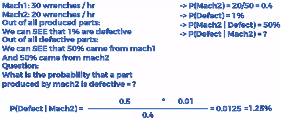
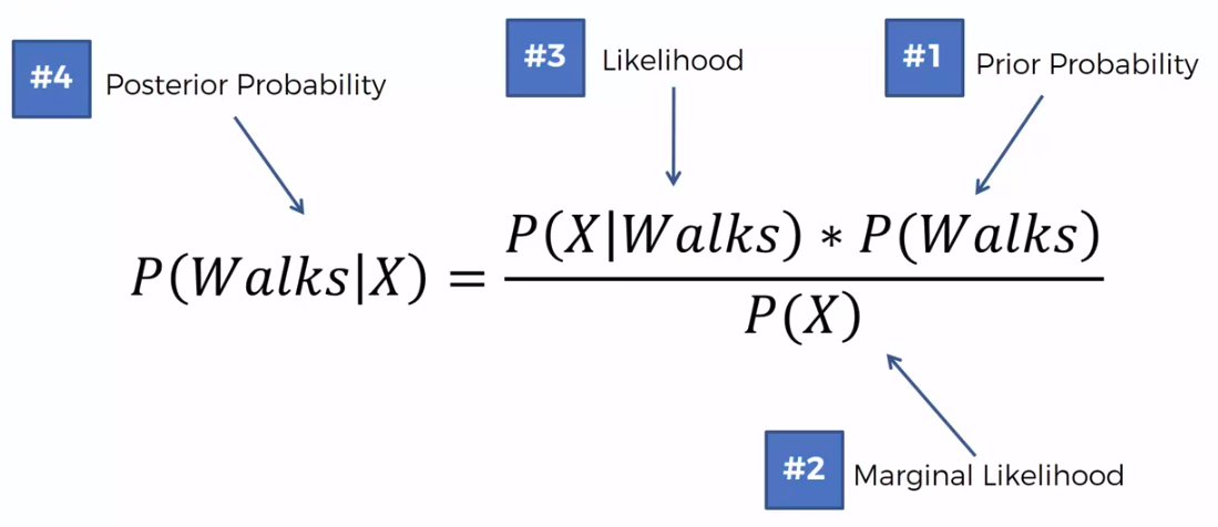
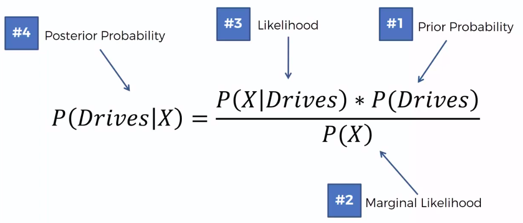
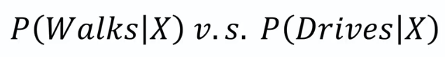
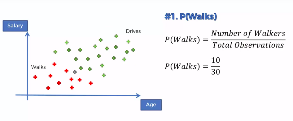
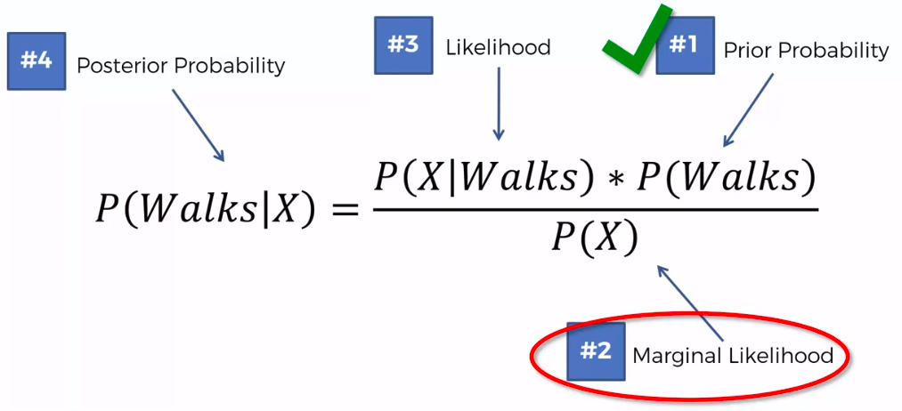
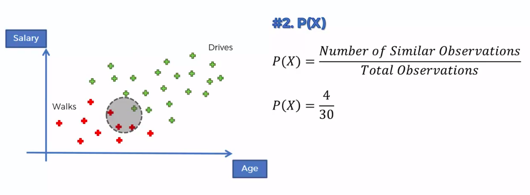
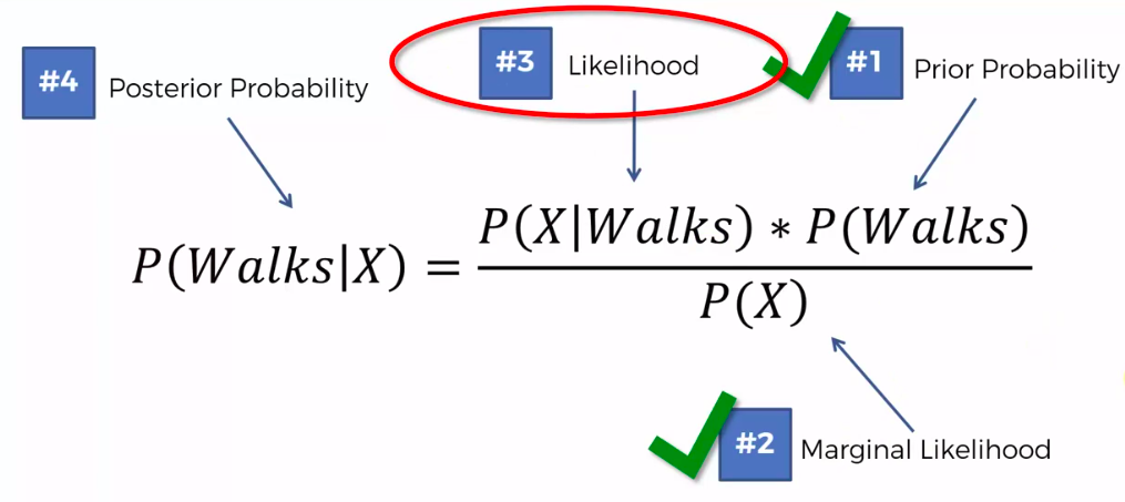
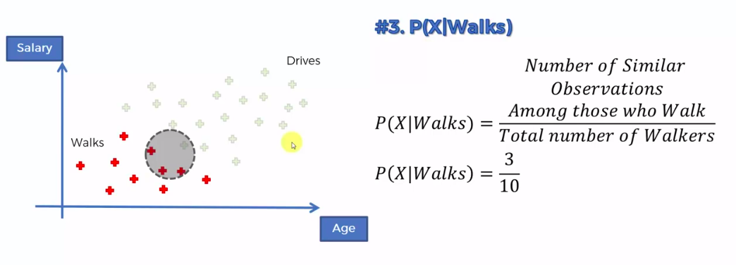
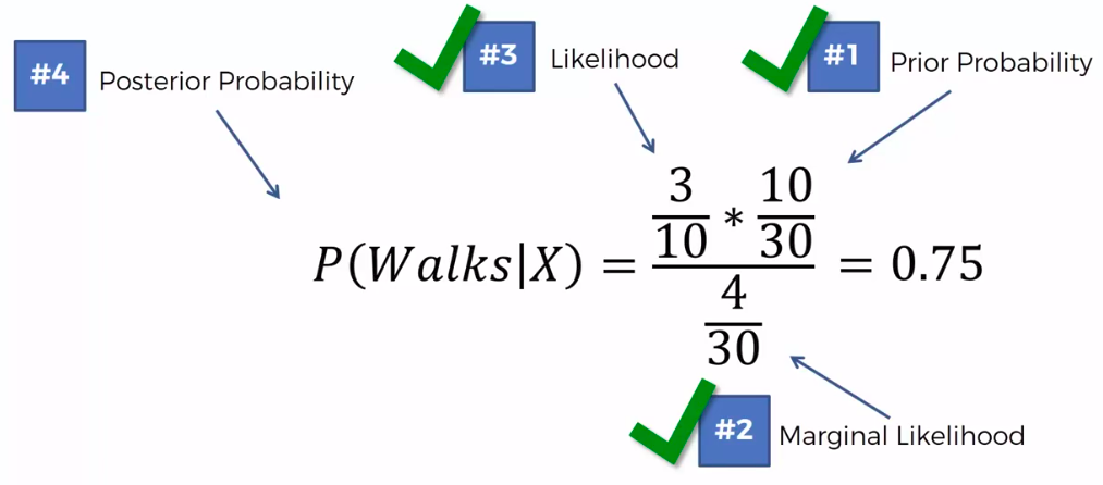
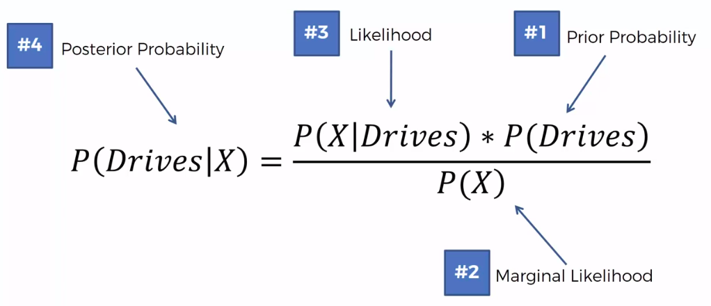
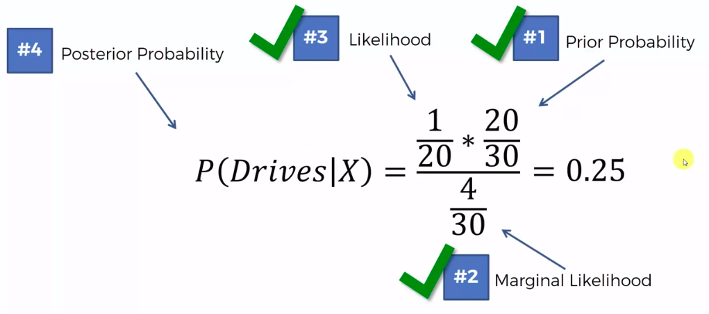
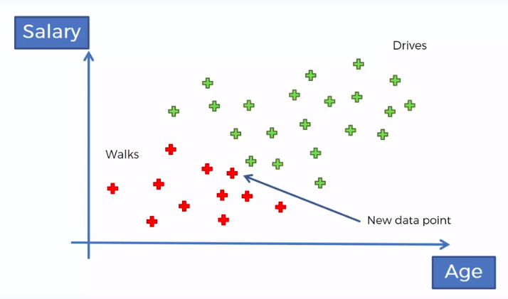
Naive Bayes
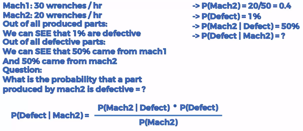
Bayes Theorem

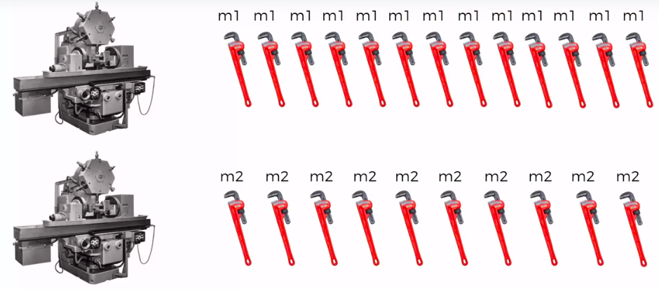
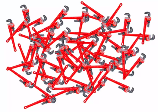
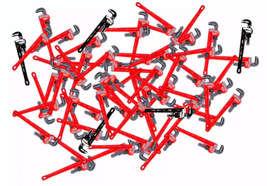
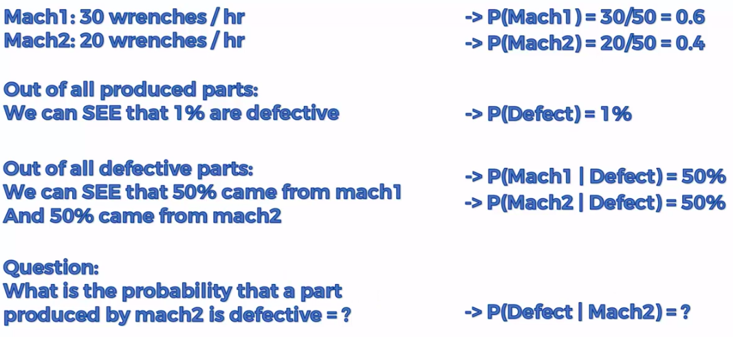
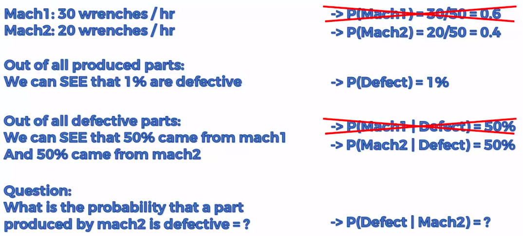
Defective Wrenche
What's the probability?
Mach1: 30 wrenches/hr
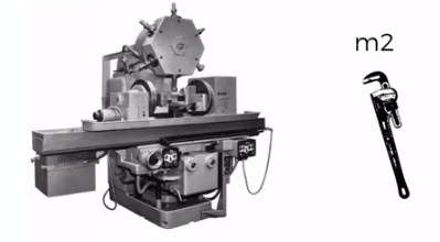
Mach2: 20 wrenches/hr
Out of all produced parts:
We can SEE that 1% are defective
Out of all defective parts:
We can SEE that 50% came from mach1 And 50% cam from mach2
Question:
What is the probability that a part produced by mach2 is defective = ?

Plan of Attack
Step 1
Step 2
Step 3
Assign class based on probability
Ready ?
Step 1
Step 1
Step 1
Step 1
Step 1
Step 1
Step 2
Step 2
Step 3
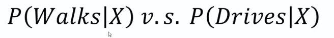
0.75 VS 0.25
0.75 > 0.25
Q: Why "Naive"?
A: Independence Assumption
Q: More than 2 features/classes?
Decision Tree
CART
Classification And Regression Trees
Classification Trees
Regression
Trees
Random Forest Classification
Ensemble Learning
Random Forest
STEP 1: Pick at random K data points from the Training set.
STEP 2: Build the tree associated to these K data points.
STEP 3: Choose the number Ntree of trees we want to build and repeat STEPS1 & 2
STEP 4: For a new data point, make each one of your Ntree trees predict value of Y to for the data point in question, and assign the new data point the average across all of the predicted Y values.

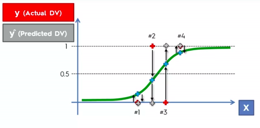
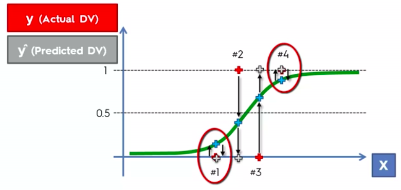
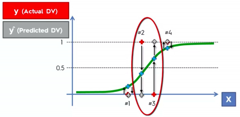
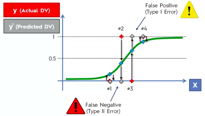
Evaluating Classifier Model Performance
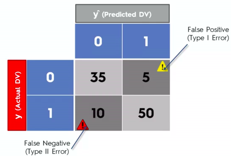
False Positives
&
False Negatives
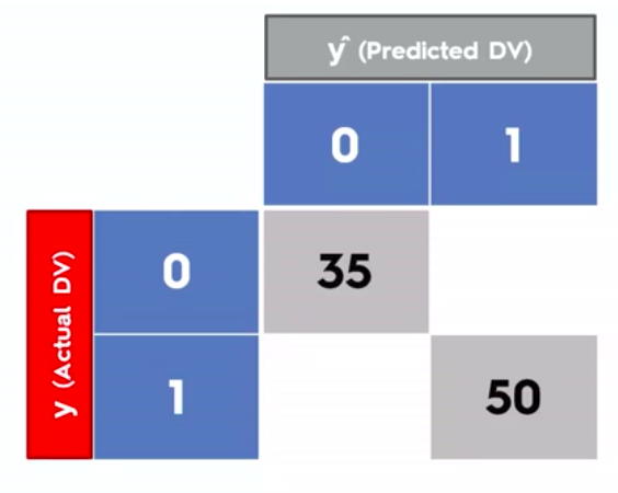
Confusion Matrix
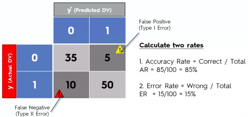
Accuracy Paradox


Classification
Model Summary
Logistic Regression
57
7
10
26
Accuracy: 83%
KNN
59
5
6
30
Accuracy: 89%
False +ve: 5
False -ve: 6
SVM (Radial)
58
6
4
32
Accuracy: 90%
False +ve: 6
False -ve: 4
Naive Bayes
57
7
7
29
Accuracy: 86%
Decision Tree
59
5
6
30
Accuracy: 83%
Random Forest
59
5
9
27
Accuracy: 86%
False +ve: 5
False -ve: 9
False +ve: 7
False -ve: 7
There is no accuracy paradox and
SVM Model is the best model for our data.
Pros and the Cons of each classification model

-
If our problem is linear, we should go for Logistic Regression or SVM.
-
If our problem is non linear, we should go for K-NN, Naive Bayes, Decision Tree or Random Forest.
- Logistic Regression or Naive Bayes when we want to rank our predictions by their probability. For example if we want to rank our customers from the highest probability that they buy a certain product, to the lowest probability. Eventually that allows us to target our marketing campaigns. And of course for this type of business problem, we should use Logistic Regression if our problem is linear, and Naive Bayes if our problem is non linear.
- SVM when we want to predict to which segment our customers belong to. Segments can be any kind of segments, for example some market segments we identified earlier with clustering.
- Decision Tree when we want to have clear interpretation of our model results,
- Random Forest when we are just looking for high performance with less need for interpretation.
Clustering
Clustering is similar to classification, but the basis is different. In Clustering we don’t know what we are looking for, and we are trying to identify some segments or clusters in our data. When we use clustering algorithms on our dataset, unexpected things can suddenly pop up like structures, clusters and groupings we would have never thought of otherwise.
K-Means Clustering
We can apply K-Means for different purposes:
- Market Segmentation,
- Medicine with for example tumor detection,
- Fraud detection
- to simply identify some clusters of your customers in your company or business.
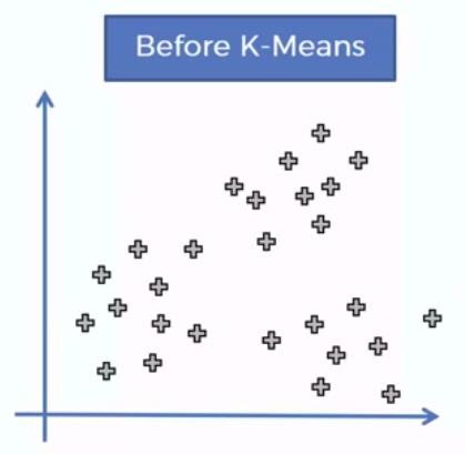
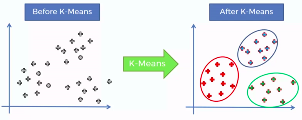
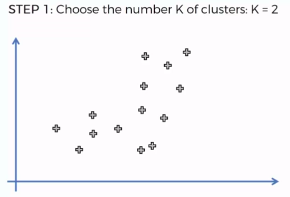
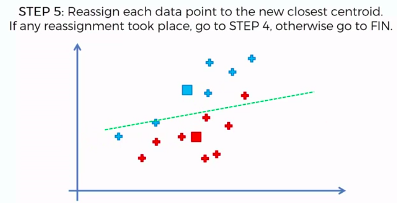
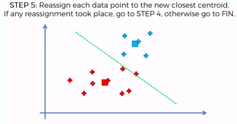
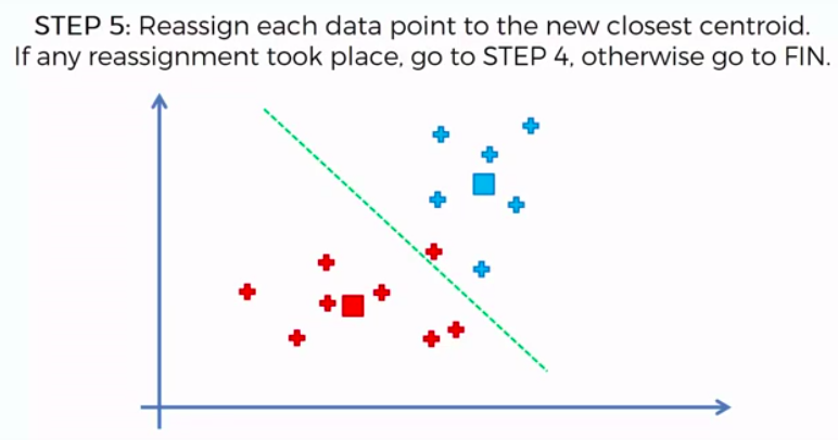
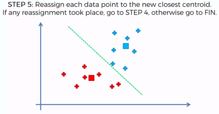
How did K-Mean did it?
STEP 1: Choose the number of K clusters
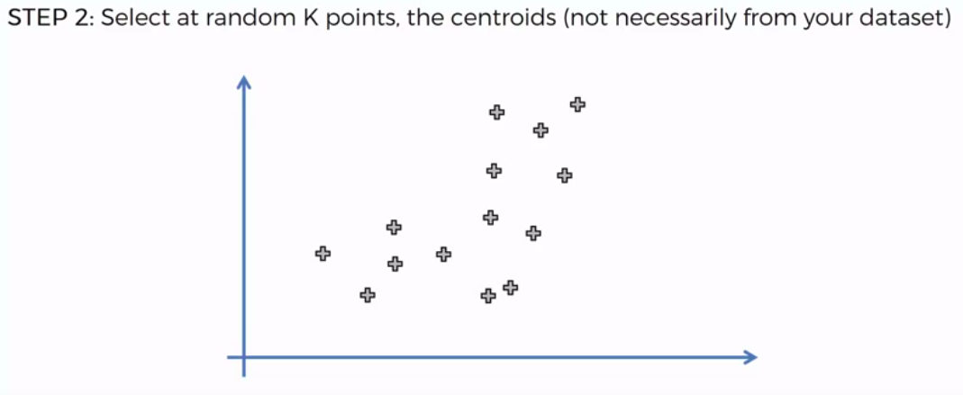
STEP 2: Select at random K points, the centroids (not necessarily from our dataset)
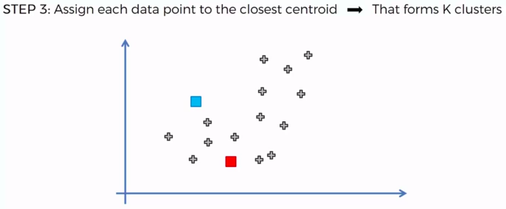
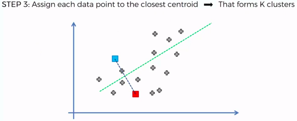
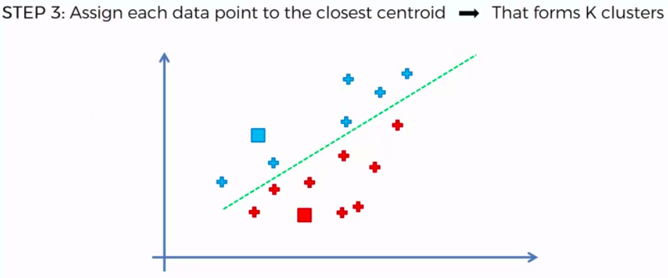
STEP 3: Assign each data point to the closest centroid -> that forms K clusters
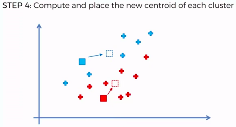
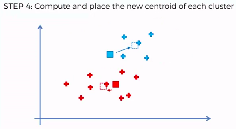
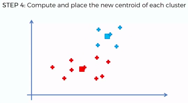
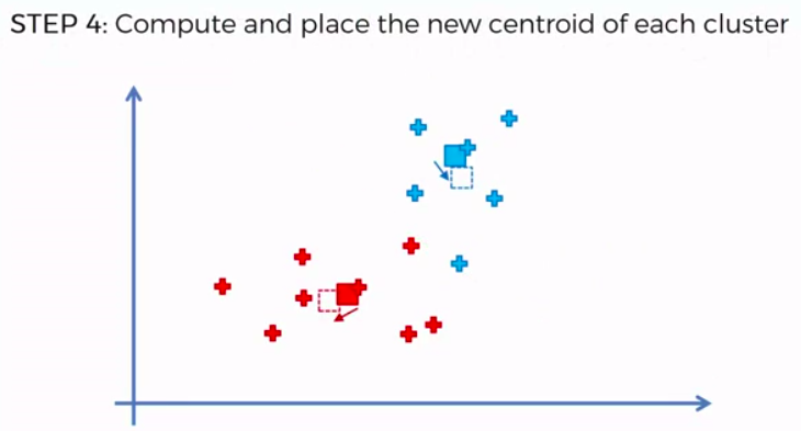
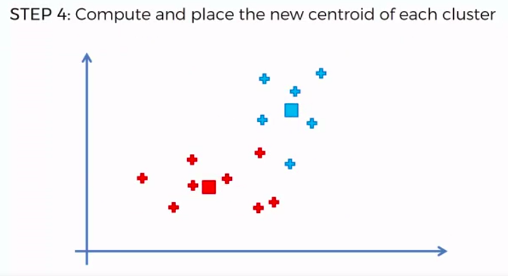
STEP 4: Compute and place the new centroid of each cluster
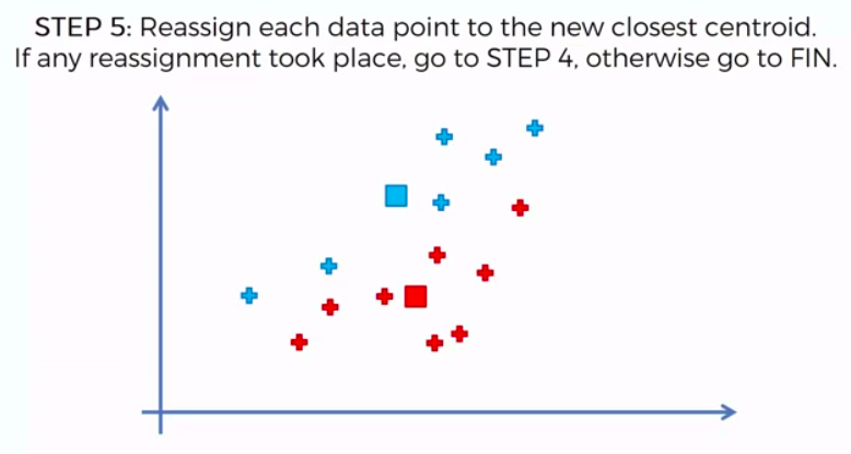
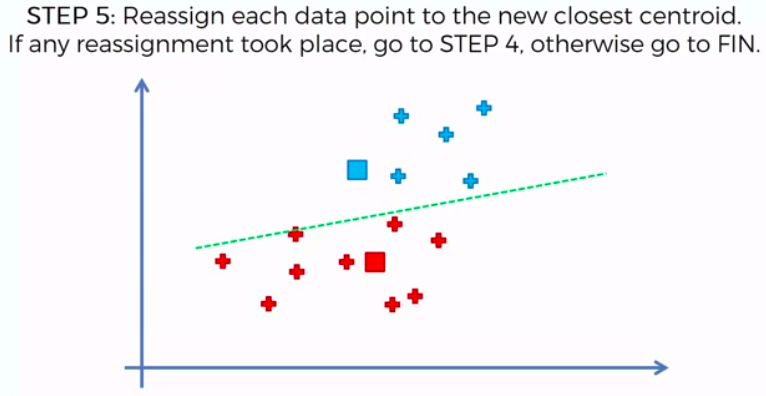
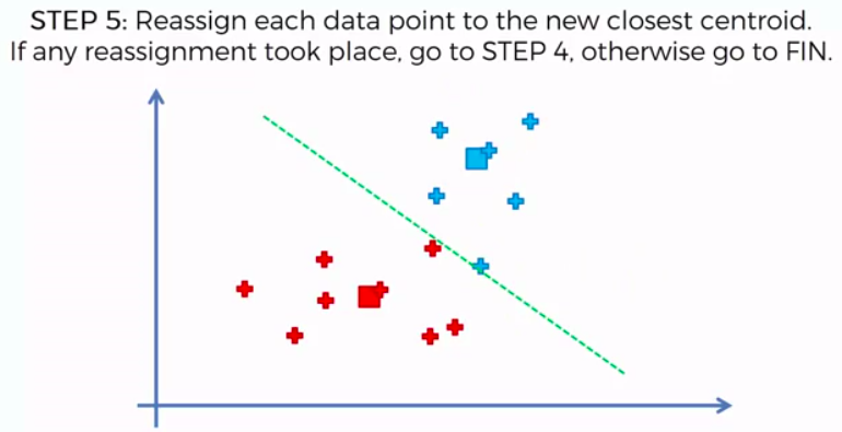
STEP 5: Reassign each data point to the new closest centroid. If any reassignment took place, go to Step 4. Otherwise go to FIN.
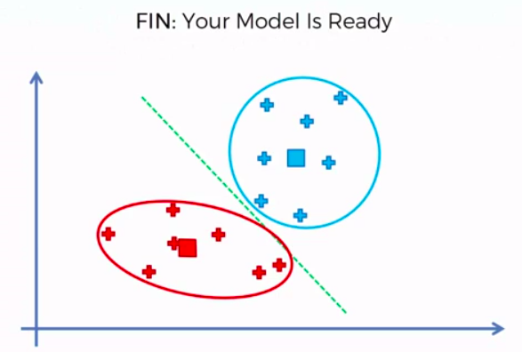
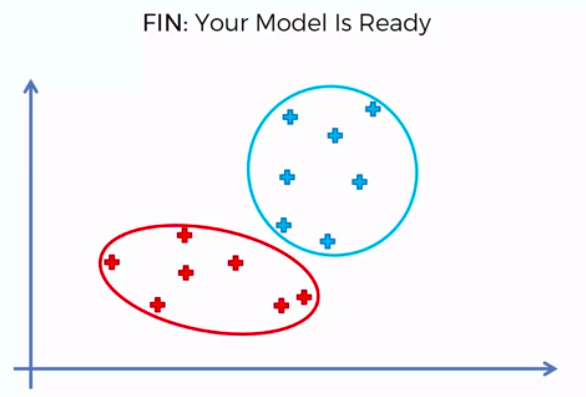
FIN: Our Model is Ready


K-Means Random Initialization Trap


What would happen if we had a bad random initialization?


Choosing the right number of clusters


A few minutes ago...


Hierarchical Clustering

2 Approach
Agglomerative
&
Divisive
Agglomerative HC
STEP 1: Make each data point a single-point cluster -> That forms N clusters
STEP 2: Take the two closest data points and make them one cluster -> That forms N-1 clusters
STEP 3: Take the two closest clusters and make them one cluster -> That forms N-2 clusters
STEP 4: Repeat STEP 3 until there is only one cluster
FIN: Our Model is Ready

Distance Between Clusters


Lets Begin !


Dendogram
How does it work?


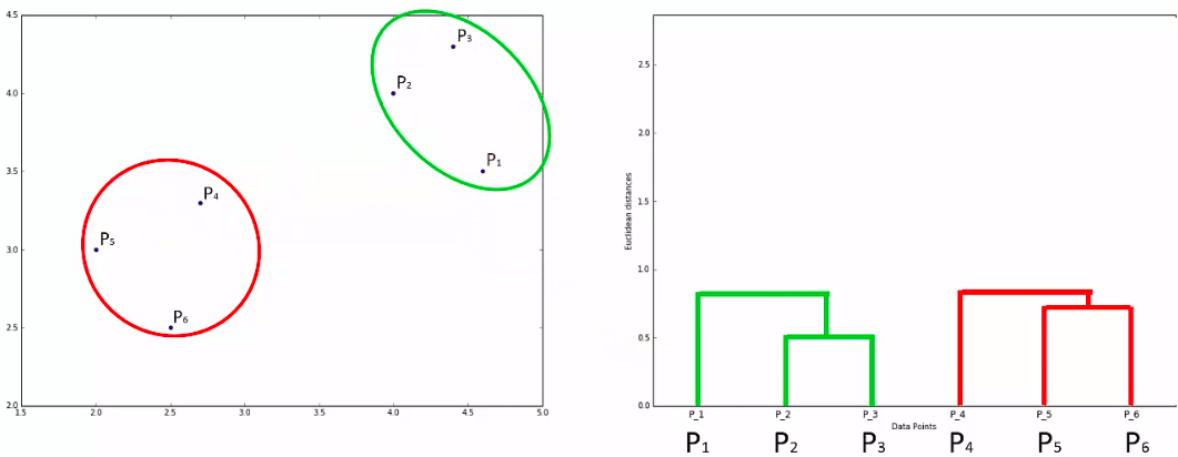

Dendogram
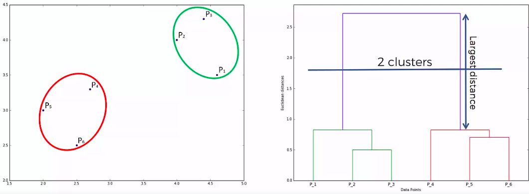
How do we use it?


Another Example:

Dendogram
get optimal number of clusters

Quiz :)


Clustering
Pros and Cons

There are no secrets to success. It is the result of preparation, hard work, and learning from failure. - Colin Powell
THANK YOU
R - Machine Learning (Intermediate)
By Abdullah Fathi
R - Machine Learning (Intermediate)
Learn how to create machine learning algorithm in R


