


federica bianco
astro | data science | data for good
dr.federica bianco | fbb.space | fedhere | fedhere
III: probability and statistics part 2
statistics
observational approach: a distribution represent the frequency with which we obtain a value ~x when measuring a phenomenon
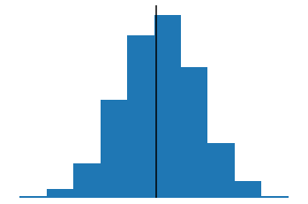
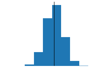
HISTOGRAMS OF SAMPLES
number of values
measured between
x and x+dx
analyst approach: a distribution represent the probability with which a phenomenon generates a value that we measure to be ~x
frequency
probability
observational approach: a distribution represent the frequency with which we obtain a value ~x when measuring a phenomenon
number of values
measured between
x and x+dx
analyst approach: a distribution represent the probability with which a phenomenon generates a value that we measure to be ~x
observational approach: a distribution represent the frequency with which we obtain a value ~x when measuring a phenomenon
number of values
measured between
x and x+dx
analyst approach: a distribution represent the probability with which a phenomenon generates a value that we measure to be ~x
frequency
probability
most common distribution:
well behaved mathematically, symmetric, when we can we will assume our uncertainties or samples are Gaussian distributed
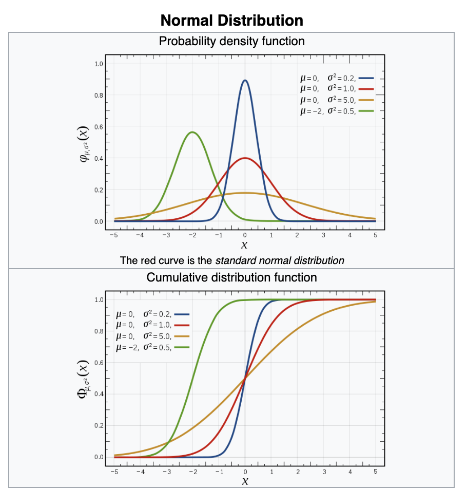
Gaussian (or normal) distribution
support: the x values for which the distribution is defined
most common distribution:
well behaved mathematically, symmetric, when we can we will assume our uncertainties or samples are Gaussian distributed
Gaussian (or normal) distribution
support: the x values for which the distribution is defined
most common distribution:
well behaved mathematically, symmetric, when we can we will assume our uncertainties or samples are Gaussian distributed
Gaussian (or normal) distribution
Central tendency
a distribution’s moments summarize its properties:
central tendency: mean (n=1)
Gaussian (or Normal) distribution
measure what fraction of a distribution is within some x values
central tendency: median (50%)
a distribution’s moments summarize its properties:
central tendency: mean (n=1)
Gaussian (or Normal) distribution
measure what fraction of a distribution is within some x values
central tendency: median (50%)
Normal
Chi-squared
a distribution’s moments summarize its properties:
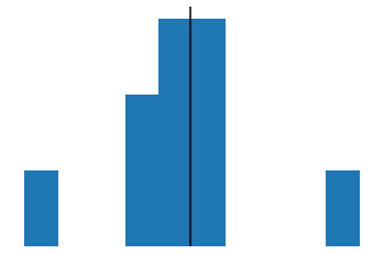
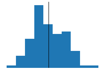
symmetric distribution: mean=median
skewed distribution: mean=median
most common distribution:
well behaved mathematically, symmetric, when we can we will assume our uncertainties or samples are Gaussian distributed
Gaussian (or normal) distribution
Spread
Normal
a distribution’s moments summarize its properties:
spread: variance (n=2)
standard deviation
measure what fraction of a distribution is within some x values
central tendency: quartiles (25%-75%)
25%-75%
Normal
a distribution’s moments summarize its properties:
spread: variance (n=2)
standard deviation
measure what fraction of a distribution is within some x values
central tendency: quantiles (5%-95%, 1%-99%...)
5%-95%
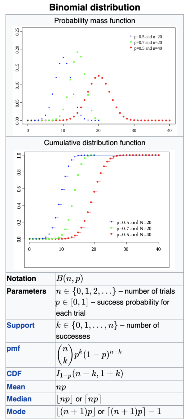
Coin toss:
Parameters: p, n
fair coin: p=0.5 n=1
Vegas coin: p=0.5 n=1
Binomial
I bet heads:
head = success
"given n tosses, each with a probability of 0.5 to get head"
Support: integer positive
Mean: np
Variance: np*(1-p)
most common distribution:
well behaved mathematically, symmetric, when we can we will assume our uncertainties or samples are Gaussian distributed
Gaussian (or normal)
distribution
Parameters: μ, σ
Support: natural numbers
Mean: μ
Variance: σ
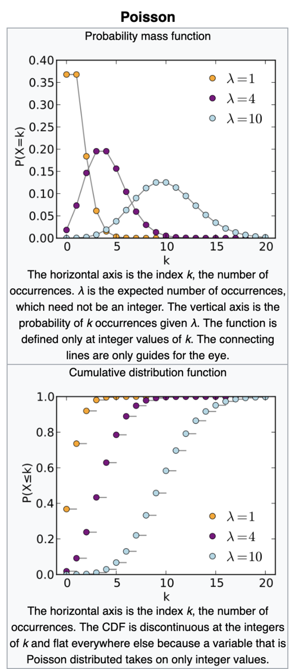
Shut noise/count noise
The innate noise in natural steady state processes (star flux, rain drops...)
Poisson
Support: natural numbers
Mean: λ
Variance: λ
Parameters: λ
a distribution’s moments summarize its properties:
central tendency: mean (n=1), median, mode (peak)
spread: standard deviation (variance n=2), quantiles
symmetry: skewness (n=3)
cuspiness: kurtosis (n=4)
Normal
Chi-squared
are they the same?
questions we need statistics to answer
videos["views"].mean()
videos["views"].median()

--> 2360784.6382573447
--> 681861.0
are these distributions the same?
if distributions have the same measured means within 1 (or n) standard deviation they should be considered "the same"
means: 1,2
standard deviation: 1,1
standard dev.
interquartile range (25%-75%)
mean
measurement uncertainty
and measurement samples
uncertainty because of the limitations of the measuring tool
uncertainty because of the limitations of the measuring tool
Take N measurements, they will all be a bit different
number of values
measured between
x and x+dx
uncertainty because of the limitations of the measuring tool
Take N measurements, they will all be a bit different
number of values
measured between
x and x+dx
uncertainty because of the limitations of the measuring tool
Take N measurements, they will all be a bit different
number of values
measured between
x and x+dx
intrinsic variance in the phenomenon
Take N measurements, they will all be a bit different
number of values
measured between
x and x+dx
Take N measurements, they will all be a bit different
number of values
measured between
x and x+dx
KEY CONCEPT:
the larger the number of samples from the distribution the more similar the distribution of our sample is to the actual "generative process": i.e. the histogram will look more and more like the actual distribution curve
THEREFORE
It is easier to tell if two distributions are the same when the samples are large
THEREFORE
I need statistical tests that acknowledge the size of the sample when I compare distributions
Law of Large Numbers
As the size of a _____________ tends to infinity the mean of the sample tends to the mean of the _______________
Laplace (1700s) but also: Poisson, Bessel, Dirichlet, Cauchy, Ellis
Let X1...XN be an N-elements sample from a population whose distribution has
mean μ and standard deviation σ
In the limit of N -> infinity
the sample mean x approaches a Normal (Gaussian) distribution with mean μ and standard deviation σ
regardless of the distribution of X
Central Limit Theorem
Easy way to assess if two number are the same:
Are the mean farther than the standard deviations?
standard deviation: 1,1
standard dev.
interquartile range (25%-75%)
mean
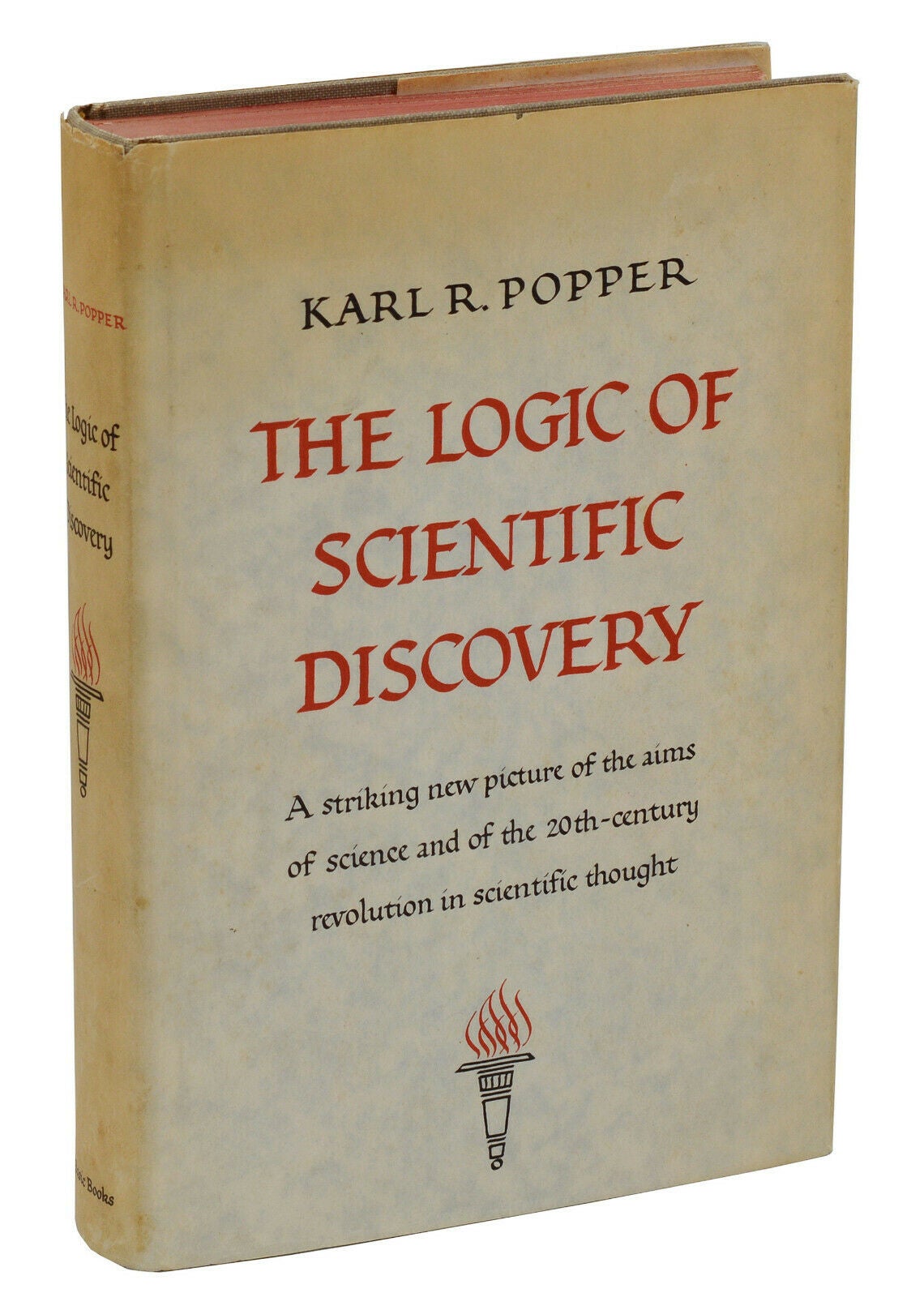
the principle of Falsifiability
3 General principles of "good" science
Falisifiability
Parsimony
Reproducibility
My proposal is based upon an asymmetry between verifiability and falsifiability; an asymmetry which results from the logical form of universal statements. For these are never derivable from singular statements, but can be contradicted by singular statements.
—Karl Popper, The Logic of Scientific Discovery
the demarcation problem:
science hypotheses needs to be falsifiable
I need to see only 1 black swan to tell that the statement that all swans are white is not true. But even if I dont see a black one it does not mean all swans are white
But what happens when I have distributions of measurements?
the demarcation problem:
science hypotheses needs to be falsifiable
Beyond any reasonable doubt
same concept guides prosecutorial justice
guilty beyond reasonable doubt
in a probabilistic sense, all hypotheses we make are possible
We will reject a hypothesis if its probability is lower than a predefined threshold
hyposthesis testing
hyposthesis testing
We do not "prove our hypothesis"
we falsify the opposite of our hypothesis
Null
Hypothesis
Rejection
Testing
formulate your prediction
Null Hypothesis
the pencils are the NOT same length (tho i think they are)
the earth is NOT round (spoiler alert... it is!!)
The NULL hypothesis is typically what I want to reject: its the way I think the world does NOT work
Null
Hypothesis
Rejection
Testing
Alternative Hypothesis
if all alternatives to our model are ruled out, then our model must hold
identify all alternative outcomes
The ALTERNATIVE hypothesis is the complete opposite of the NULL
Null
Hypothesis
Rejection
Testing
confidence level
p-value
threshold
set confidence threshold
95%
Null
Hypothesis
Rejection
Testing
find a measurable quantity which under the Null has a known distribution
Null
Hypothesis
Rejection
Testing
find a measurable quantity which under the Null has a known distribution
if the Null hypothesis holds
Null
Hypothesis
Rejection
Testing
find a measurable quantity which under the Null has a known distribution
For example, it follows a Gaussian Distribution with mean 0 and standard deviation 1
Null
Hypothesis
Rejection
Testing
find a measurable quantity which under the Null has a known distribution
if a quantity follows a known distribution, once I measure its value I can what the probability of getting that value actually is! was it a likely or an unlikely draw?
if my quantity is ~20 its very likely
if my quantity is ~35 its very unlikely
Null
Hypothesis
Rejection
Testing
also called "statistics"
e.g.: Z statistics: difference between means ~N(0,1)
χ2 statistics: difference between prediction and reality squared ~
K-S statistics: maximum distance of cumulative distributions
Null
Hypothesis
Rejection
Testing
The distribution of sample means for (independent) samples extracted from a population
with mean μ and standard deviation σ is
Normally distributed
If I measure the mean of two samples
(the samples of pencil measurements)
I expect the difference to be a number drawn from a standard normal: Gaussian w mean 0 variance 1
Highest prob. is 0
Prob that the number is within 1σ of the mean is 68%
If the means are within 1-sigma of each other that means that I cannot rule out that the distributions are the same to a 1-sigma level (p-value 0.32)
If the means are not 1-sigma of each other that means that I can rule out that the distributions are the same to a 1-sigma level (p-value 0.32)
reject the null
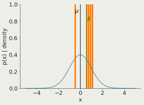
Is the mean of a sample with known variance the same as that of a known population?
sample mean
sample variance =
population mean
Is the mean of a sample with known variance the same as that of a known population?
sample mean
sample variance =
population mean
The Z test -meaning the statistic is ~N(0,1)-
provides a trivial interpretation of the measured quantity:
the Z value is exactly the distance for the mean of the standard distribution of possible outcomes in units of standard deviation
so a result of 0.13 means we are 0.13 standard deviations to the mean (p>0.05)
sample variance =
population mean
Is the mean of a sample with known variance the same as that of a known population?
sample mean
sample variance =
population mean
why do we need a test? why not just measuring the means and seeing it they are the same?
sample variance =
population mean
Null
Hypothesis
Rejection
Testing
calculate it!
Null
Hypothesis
Rejection
Testing
test data against alternative outcomes
95%
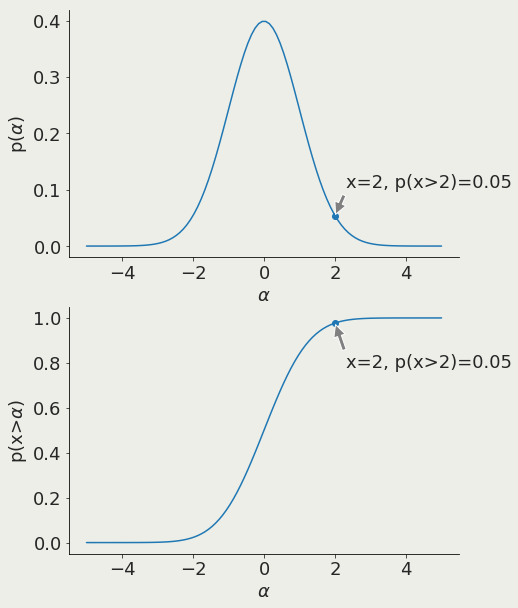
α is the x value corresponding to a chosen threshold
if its a Z test the number i get is the distance from the mean in units of standard deviation
Null
Hypothesis
Rejection
Testing
test data against alternative outcomes
prediction is unlikely
Null rejected
Alternative holds
Null
Hypothesis
Rejection
Testing
test data against alternative outcomes
prediction is unlikely
Null rejected
Alternative holds
this corresponds to measuring a valu of the statistics in the tail of the distribution
Null
Hypothesis
Rejection
Testing
test data against alternative outcomes
prediction is likely
Null holds for now
prediction is unlikely
Null rejected
Alternative holds
95%
Null
Hypothesis
Rejection
Testing
test data against alternative outcomes
prediction is likely
Null holds for now
prediction is unlikely
Null rejected
Alternative holds
95%
data
does not falsify alternative
falsifies alternative
model
holds
"Under the Null Hypothesis" = if the proposed model is false
this has a low probability of happening
model
prediction
everything but model is rejected
low probability event happened
formulate the Null as the comprehensive opposite of your theory
Key Slide
formulate your prediction (NH)
identify all alternative outcomes (AH)
set confidence threshold
(p-value)
find a measurable quantity which under the Null has a known distribution
(pivotal quantity)
calculate the pivotal quantity
calculate probability of value obtained for the pivotal quantity under the Null
if probability < p-value : reject Null
Key Slide
p-value hypothesis testing
5
Imagine that I take a measurements of a quantity that is expected to be normally distributed with mean 0 and stdev 1
what is the probability that I would measure 1.5?
16%
16%
The probability of measuring any one value is mathematically 0... however I can say that
the probability of measuring something between -1σ and 1σ (within 1-sigma) is 68%.
So the probability of measuring something outside is 100-68 = 32%.
So if I measure something outside of [-1σ:1σ] that had a probability <32% of being measured.
Imagine that I take a measurements of a quantity that is expected to be normally distributed with mean 0 and stdev 1
what is the probability that I would measure 1.5?
The probability of measuring any one value is mathematically 0... however I can say that
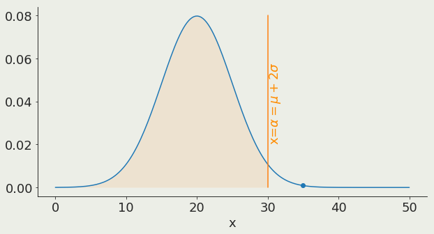
the probability of measuring something between -2σ and 2σ (within 2-sigma) is 95%.
So the probability of measuring something outside is 100-95 = 5%.
So if I measure something outside of [-2σ:2σ] that had a probability <5% of being measured.
Imagine that I take a measurements of a quantity that is expected to be normally distributed with mean 0 and stdev 1
what is the probability that I would measure 1.5?
The probability of measuring any one value is mathematically 0... however I can say that
the probability of measuring something between -3σ and 3σ (within 3-sigma) is 99.7%.
So the probability of measuring something outside is 100-99.7 = 0.3%.
So if I measure something outside of [-3σ:3σ] that had a probability <0.3% of being measured.
Imagine that I take a measurements of a quantity that is expected to be normally distributed with mean 0 and stdev 1
what is the probability that I would measure 1.5?
it might be easier to think about it as cumulative distributions if you are comfortable with integrals
the probability of measuring something between -3σ and 3σ (within 3-sigma) is 99.7%.
So the probability of measuring something outside is 100-99.7 = 0.3%.
So if I measure something outside of [-3σ:3σ] that had a probability <0.3% of being measured.
Distribution of measurements under the Null hypothesie
2σ
Null hypothesis cannot be rejected at a
p-value 0.05
p-value hypothesis testing
step by step
6
set up threshold α
its important to do this first. If we do not we may be tempted to choose a threshold that fits our result, thus always reporting rejection of null hypothesis
set up threshold α
identify how you expect your measurement to be distributed under the Null hypothesis
set up threshold α
identify how you expect your measurement to be distributed under the Null hypothesis
measure outcome from data: x0
set up threshold α
identify how you expect your measurement to be distributed under the Null hypothesis
falsify H0
measure outcome from data: x0
H0 cannot be falsified
set up threshold α
identify how you expect your measurement to be distributed under the Null hypothesis
falsify H0
measure outcome from data: x0
H0 cannot be falsified
this quantity is called a "statistics"
p-value hypothesis testing
common tests
6
Statistical way to measure differences:
In NHRT a statistics is a quantity that relates to the data which has a known distribution under the Null Hypothesis
In NHRT a statistics is a quantity that relates to the data which has a known distribution under the Null Hypothesis
e.g.: Z statistics is Normally distributed Z~N(0,1)
In absence of effect (i.e. under the Null)
== the sample mean is the same as the population mean
Z is distributed according to a Gaussian N(μ=0, σ=1)
Does a sample come from a known population?
Example: new bus route implementation.
https://github.com/fedhere/PUS2022_FBianco/blob/master/classdemo/ZtestBustime.ipynb
You know the mean and standard deviation of a but travel route: that is the population
You measure the new travel time between two stops 10 times: that is your sample.
Has travel time changed?
2σ
95%
Z -test
In absence of effect (i.e. under the Null)
== the sample mean is the same as the population mean
Z is distributed according to a Gaussian N(μ=0, σ=1)
2σ
95%
The expectation is that Z will be distributed following a standard normal: a Gaussian with mean 0 std 1.
Values away from 0 are increasingly less probable.
68% probability to get a number b/w -1 and +1
95% probability to get a number b/w -2 and +2
How to interpret the number you get?
Does a sample come from a known population?
Z -test
In absence of effect (i.e. under the Null)
== the sample mean is the same as the population mean
Z is distributed according to a Gaussian N(μ=0, σ=1)
2σ
95%
IF OUR p-value THRSHOLD IS 1-sigma that means the 68% region is between -1 and +1
=> We have less 68% probability of getting a number <-1 or > 1
How to interpret the number you get?
Does a sample come from a known population?
Z -test
In absence of effect (i.e. under the Null)
== the proportions of men and women are the same
Z is distributed according to a Gaussian N(μ=0, σ=1)
Are 2 proportions (fractions) the same?
Example: citibike women usage patterns
https://github.com/fedhere/PUS2020_FBianco/blob/master/classdemo/citibikes_gender.ipynb
You want to know if women are less likely than man to use citibike to commute.
You know the fraction of rides women (men) take during the week
2σ
95%
Z -test
In absence of effect (i.e. under the Null)
== the proportions of men and women are the same
Z is distributed according to a Gaussian N(μ=0, σ=1)
2σ
95%
Are 2 proportions (fractions) the same?
Z -test
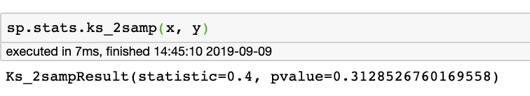
Kolmogorof-Smirnoff :
do two samples come from the same parent distribution?
Cumulative distribution 1
Cumulative distribution 2
Kolmogorof-Smirnoff :
do two samples come from the same parent distribution?
Cumulative distribution 1
Cumulative distribution 2
uncertainty
model
observation
number of observation
this should actually be the number of params in the model
are the data what is expected from the model (if likelihood is Gaussian... we'll see this later) - ther are a few χ2 tests. The one here is the "Pearson's χ2 tests"
uncertainty
model
observation
number of observation
are the data what is expected from the model (if likelihood is Gaussian... we'll see this later) - ther are a few χ2 tests. The one here is the "Pearson's χ2 tests"
In absence of effect (i.e. under the Null)
== the samples are drawn from the same population
The KS test is chi-square distributed
Are 2 samples the same?
KS-test
In absence of effect (i.e. under the Null)
== the samples are drawn from the same population
The KS test is chi-square distributed
Cumulative distribution 1
Cumulative distribution 2
Are 2 samples the same?
KS-test
Cumulative distribution 1
Cumulative distribution 2
Are 2 samples the same?
KS-test
Cumulative distribution 1
Cumulative distribution 2
Are 2 samples the same?
KS-test
Statistics and tests
Types of Data:
Data Definitions
Data: observations that have been collected
Population: the complete body of subjects we want to infer about
Sample: the subset of the population about which data is collected/available
Census: collection of data from the entire population
Parameter: the subset of the population we actually studied collection of data from the entire population
Statistics: numerical value describing an attribute of the population numerical value describing an attribute of the sample
Data Definitions
The analysis of our ______
showed that for our 10 _________ the mean income is $60k. The standard deviation of the ______ means is $12k. From this _______ we infer for the _____________ a mean income _________ $60k +/- $12k
data
sample
statistics
population
parameter
data kinds and nomenclature
7
At the root is the fact that a sample drawn from a parent distribution will look increasingly more like the parent distribution as the size of the sample increases.
More formally: The distribution of the means of N samples generated from the same parent distribution will
I. be normally distributed (i.e. will be a Gaussian)
II. have mean equal to the mean of the parent distribution, and
III. have standard deviation equal to the parent population standard deviation divided by the square root of the sample size
Qualitative variables
No ordering
UrbanScience e.g. precinct, state, gender, Also called Nominal, Categorical
Types of Data:
Qualitative variables
No ordering
UrbanScience e.g. precinct, state, gender, Also called Nominal, Categorical
Types of Data:
Qualitative variables
No ordering
UrbanScience e.g. precinct, state, gender, Also called Nominal, Categorical
Quantitative variables
Ordering is meaningful
Time, Distance, Age, Length, Intensity, Satisfaction, Number of
Types of Data:
Qualitative variables
No ordering
UrbanScience e.g. precinct, state, gender, Also called Nominal, Categorical
Quantitative variables
Ordering is meaningful
Time, Distance, Age, Length, Intensity, Satisfaction, Number of
Counts:
number of people in a county
Ordinal:
survey response Good/Fair/Poor
discrete
Types of Data:
Qualitative variables
No ordering
UrbanScience e.g. precinct, state, gender, Also called Nominal, Categorical
Quantitative variables
Ordering is meaningful
Time, Distance, Age, Length, Intensity, Satisfaction, Number of
continuous
Counts:
number of people in a county
Ordinal:
survey response Good/Fair/Poor
Continuous
Ordinal:
Earthquakes (notlinear scale)
Interval:
F temperature interval size preserved
Ratio:
Car speed
0 is naturally defined
discrete
Types of Data:
Qualitative variables
No ordering
UrbanScience e.g. precinct, state, gender, Also called Nominal, Categorical
Quantitative variables
Ordering is meaningful
Time, Distance, Age, Length, Intensity, Satisfaction, Number of
continuous
Counts:
number of people in a county
Ordinal:
survey response Good/Fair/Poor
Interval:
F temperature interval size preserved
Ratio:
Car speed
0 is naturally defined
discrete
Censored: age>90
Missing: “Prefer not to answer” (NA / NaN)
Types of Data:
Continuous
Ordinal:
Earthquakes (notlinear scale)
descriptive statistics
null hypothesis rejection testing setup
pivotal quantities
Z, K-S tests
By federica bianco
Foundations of Data Science for Everyone - Probability and Statistics


