foundations of data science for everyone VII

dr.federica bianco | fbb.space |    fedhere |    fedhere

Tree methods

this slide deck:

https://slides.com/federicabianco/fdsfe_7

Machine Learning basic concepts
- interpretability
- parameters vs hyperparameters
- supervised/unsupervised

Tree methods
- single trees
- hyperparameters
- weaknesses

Tree ensembles
Feature importance
Categorical feature encoding
ML models performance evaluation

recap

what is machine learning

what is machine learning?

classification

prediction

feature selection

supervised learning

understanding structure

organizing/compressing data

anomaly detection dimensionality reduction

unsupervised learning

clustering

PCA

Apriori

k-Nearest Neighbors

Regression

Support Vector Machines

Classification/Regression Trees

Neural networks

Clustering

partitioning the feature space so that the existing data is grouped (according to some target function!)

Classifying & regression

finding functions of the variables that allow to predict unobserved properties of new observations

Unsupervised learning

understanding structure
anomaly detection
dimensionality reduction

All features are observed for all datapoints

unsupervised vs supervised learning

prediction and classification based on examples

All features are observed for all datapoints

Some features can't be observed

for some datapoints

0.1 classification

classifying:

supervised learning

observed features:

(x, y)

models typically return a partition of the space

goal is to partition the space so that the unobserved variables are

separated in groups

consistently with

an observed subset

target features:

(color)

observed features:

(x, y)

ax+b

if y <= a*x + b :
	return blue
else:
	return orange

target features:

(color)

classifying:

supervised learning

observed features:

(x, y)

if x**2 + y**2 <= (x-a)**2 + (y-b)**2 :
	return blue
else:
	return orange

target features:

(color)

classifying:

supervised learning

observed features:

(x, y)

if x**2 + y**2 <= (x-a)**2 + (y-b)**2 :
	return blue
else:
	return orange

target features:

(color)

classifying:

supervised learning

observed features:

(x, y)

this is a solution SVM would provide:

Support Vector Machine

target features:

(color)

classifying:

supervised learning

observed features:

(x, y)

supervised ML: classification

Support Vector Machine:

finds a hyperplane that partitions the space

A subset of variables has class labels. Guess the label for the other variables

target features:

(color)

observed features:

(x, y)

supervised ML: classification

Support Vector Machine:

finds a hyperplane that partitions the space

A subset of variables has class labels. Guess the label for the other variables

2d hyperplane: line (curve)

3d hyperplane: surface

4d hyperplane: volume

...

target features:

(color)

observed features:

(x, y)

supervised ML: classification

Tree Methods

split spaces along each axis separately

A subset of variables has class labels. Guess the label for the other variables

target features:

(color)

observed features:

(x, y)

supervised ML: classification

Tree Methods

split spaces along each axis separately

A subset of variables has class labels. Guess the label for the other variables

split along x

if x <= a :
	return blue
else:
	return orange

target features:

(color)

observed features:

(x, y)

supervised ML: classification

Tree Methods

split spaces along each axis separately

A subset of variables has class labels. Guess the label for the other variables

split along x

if x <= a :
	if y <= b:
      		return blue
return orange

then

along y

target features:

(color)

0.2 ML model performance

Accuracy

Predicted

Actual

232

263

negative

positive

negative

positive

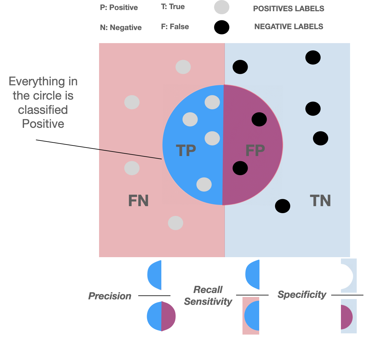
Classification outcomes:

true positives (TP) : "+" correctly labeled as "+"

true negatives (TN) : "-" correctly labeled as "-"

false positives (FP) : "-" incorrectly labeled as "+"

false negatives (FN) : "+" incorrectly labeled as "-"

accuracy:

\frac{TP+TN}{N} = \frac{TP+TN}{TP+FP+TN+FN}

accuracy =

\frac{232+263}{500}=99\%

Precision and Recall

precision:

(or specificity)

recall:

(or sensitivity)

\frac{TP}{TP+FP}

\frac{TP}{TP+FN}

Fraction of objects you think are positive that actually are positive

Fraction of positive objects that you were able to find

F1-score:

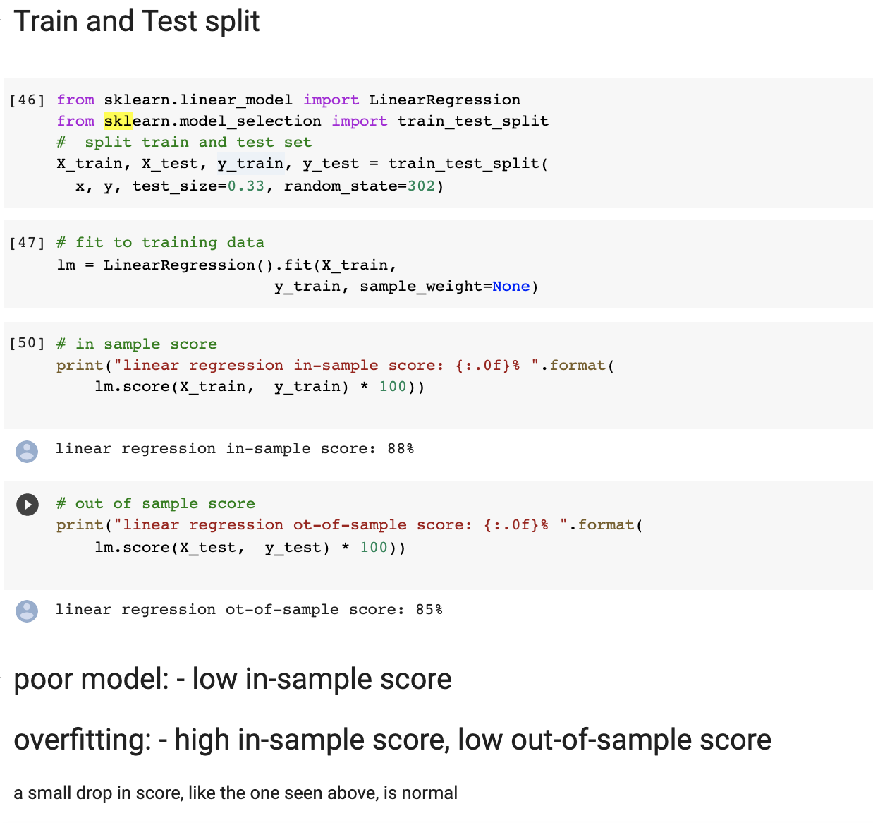
\frac{2\times\text{ precision }\times\text{ recall}}{\text{precision }+\text{ recall}}

Training and testing

263

Wnen we want to train a model to predict we
SPLIT THE DAT INTO 2 or 3 SETS

training:

we use it to train the model

testing:

we use it to test the model.

we use the test set to report our result

Predicted

Actual

220

253

negative

positive

accuracy =

\frac{220+253}{500}=95\%

Predicted

Actual

232

263

negative

positive

negative

positive

accuracy =

\frac{232+263}{500}=99\%

negative

ideally the model performer as well on the testing as training
if it performs much worse its a sign of overfitting

Cross validation

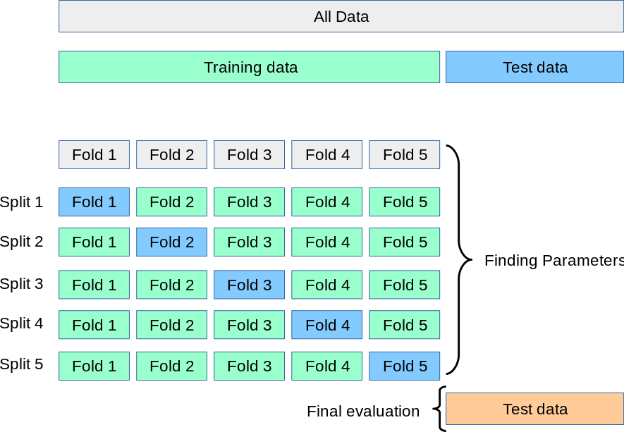
test train validation

train parameters on training set

run only once on the test set to assess the model performance

Cross validation

test + train + validation

train parameters on training set

adjust parameters on validation set

run only once on the test set to assess the model performance

Cross validation

k-fold cross validation

Higher level metrics

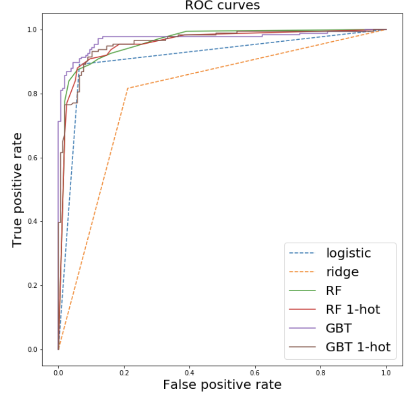
ROC: Receiver Operator Characteristics Curve

AUC: Area Under the Curve

Receiver operating characteristic

GOOD

BAD

tuning models by changing hyperparameters

(e.g. threshold)

Receiver operating characteristic

For probabilistic models where you can choose a threshold for "positive": every threshold pputs a point in this plot

positive iff p(positive) > threshold

Receiver operating characteristic

For probabilistic models where you can choose a threshold for "positive": every threshold pputs a point in this plot

threshold ~1.0: everything is negative

threshold ~0.0 : everythong is positive

positive iff p(positive) > threshold

Receiver operating characteristic

GOOD

BAD

Receiver operating characteristic

AUC: Area Under the Curve

a global assessment of the potential of the model

AUC: Area Under the Curve

a global assessment of the potential of the model

the larger the area the better

Receiver operating characteristic

a global assessment of the potential of the model

AUC: Area Under the Curve

a global assessment of the potential of the model

AUC: Area Under the Curve

a global assessment of the potential of the model

the larger the area the better

Tree Methods

supervised learning method

partitions feature space along each feature separately

The good

Non-Parametric
White-box: can be easily interpreted
Works with any feature type and mixed feature types
Works with missing data
Robust to outliers

The bad

High variability (-> use ensamble methods)
Tendency to overfit
(not really easily interpretable after all...)

1 single tree

(Kaggle)

Application:

a robot to predict surviving the Titanic

714 passengers Ns=424 Nd=290

https://www.kaggle.com/c/titanic

features:

gender
ticket class
age

target variable:

-> survival (y/n)

gender (binary)

Ns=93 Nd=360

Ns=197 Nd=64

(Kaggle)

Application:

a robot to predict surviving the Titanic

https://www.kaggle.com/c/titanic

features:

gender
ticket class
age

target variable:

-> survival (y/n)

gender (binary)

Ns=93 Nd=360

Ns=197 Nd=64

optimize over purity:

p~ = ~\frac{N_{largest~class}}{N_{total}}

714 passengers Ns=424 Nd=290

(Kaggle)

Application:

a robot to predict surviving the Titanic

https://www.kaggle.com/c/titanic

features:

gender
ticket class
age

target variable:

-> survival (y/n)

gender (binary)

Ns=93 Nd=360

Ns=197 Nd=64

optimize over purity:

p~ = ~\frac{N_{largest~class}}{N_{total set}}

p=\frac{360}{360+93}

p=\frac{197}{197+64}

714 passengers Ns=424 Nd=290

(Kaggle)

Application:

a robot to predict surviving the Titanic

https://www.kaggle.com/c/titanic

features:

gender
ticket class
age

target variable:

-> survival (y/n)

gender (binary)

Ns=93 Nd=360

Ns=197 Nd=64

optimize over purity:

p~ = ~\frac{N_{largest~class}}{N_{total set}}

p= 79\%

p=75\%

714 passengers Ns=424 Nd=290

(Kaggle)

Application:

a robot to predict surviving the Titanic

https://www.kaggle.com/c/titanic

features:

gender 79%|75%
ticket class 66 | 54%
age

target variable:

-> survival (y/n)

1st

Ns=120 Nd=80

2nd +3rd

Ns=234 Nd=298

p= 66\%

p=54\%

class (ordinal)

714 passengers Ns=424 Nd=290

(Kaggle)

Application:

a robot to predict surviving the Titanic

https://www.kaggle.com/c/titanic

features:

gender 79%|75%
ticket class 66% | 54%
age 66% | 61%

target variable:

-> survival (y/n)

age (continuous)

>6.5

Ns=250 Nd=107

<=6.5

Ns=139 Nd=217

714 passengers Ns=424 Nd=290

(Kaggle)

Application:

a robot to predict surviving the Titanic

https://www.kaggle.com/c/titanic

features:

gender 79%|75%
ticket class 66% | 44%
age 66% | 61%

target variable:

-> survival (y/n)

age (continuous)

>6.5

Ns=250 Nd=107

<=6.5

Ns=139 Nd=217

714 passengers Ns=424 Nd=290

(Kaggle)

Application:

a robot to predict surviving the Titanic

https://www.kaggle.com/c/titanic

target variable:

-> survival (y/n)

gender (binary)

Ns=93 Nd=360

Ns=197 Nd=64

features:

gender 79|75%
ticket class M 60|85% F 96|65%
age M 74|67% F 66|60%

714 passengers Ns=424 Nd=290

(Kaggle)

Application:

a robot to predict surviving the Titanic

https://www.kaggle.com/c/titanic

target variable:

-> survival (y/n)

gender (binary)

Ns=93 Nd=360

Ns=197 Nd=64

features:

gender 79|75%
ticket class M 60|85% F 96|65%
age M 74|67% F 66|60%

714 passengers Ns=424 Nd=290

(Kaggle)

Application:

a robot to predict surviving the Titanic

https://www.kaggle.com/c/titanic

target variable:

-> survival (y/n)

gender

Ns=93 Nd=360

Ns=197 Nd=64

age

>6.5

Ns=250 Nd=107

<=6.5

Ns=139 Nd=217

class

1st + 2nd

Ns=120 Nd=80

3rd

Ns=234 Nd=298

features:

gender 79|75%
ticket class M 60|85% F 96|65%
age M 74|67% F 66|60%

714 passengers Ns=424 Nd=290

(Kaggle)

Application:

a robot to predict surviving the Titanic

https://www.kaggle.com/c/titanic

target variable:

-> survival (y/n)

gender

Ns=93 Nd=360

Ns=197 Nd=64

age

>6.5

Ns=250 Nd=107

p=82%

<=6.5

Ns=139 Nd=217

p=67%

class

age

>2.5

Ns=1 Nd=1

p=50%

<=2,5

Ns=8 Nd=139

p=95%

age

>38.5

Ns=44 Nd=46

<=38.5

Ns=11 Nd=1

1st + 2nd

Ns=120 Nd=80

3rd

Ns=234 Nd=298

features:

gender 79|75%
ticket class M 60|85% F 96|65%
age M 74|67% F 66|60%

714 passengers Ns=424 Nd=290

(Kaggle)

Application:

a robot to predict surviving the Titanic

https://www.kaggle.com/c/titanic

features:

gender (binary already used)
ticket class (ordinal)
age (continuous)

target variable:

-> survival (y/n)

gender

Ns=93 Nd=360

Ns=197 Nd=64

>6.5

Ns=250 Nd=107

p=82%

<=6.5

Ns=139 Nd=217

p=67%

1st + 2nd

Ns=120 Nd=80

3rd

Ns=234 Nd=298

1st

Ns=100 Nd=20

p=80%

2nd

Ns=40 Nd=40

p=50%

age

>38.5

Ns=44 Nd=46

<=38.5

Ns=11 Nd=1

class

age

class

714 passengers Ns=424 Nd=290

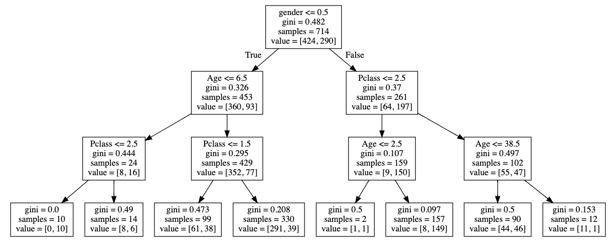
A single tree

nodes

(make a decision)

root node

branches

(split off of a node)

leaves (last groups)

https://github.com/fedhere/DSPS/blob/master/lab9/titanictree.ipynb

A single tree

this visualization is called a "dendrogram"

2 tree hyperparameters

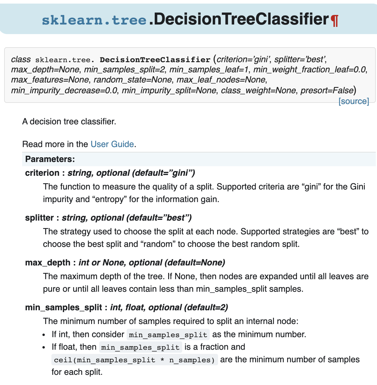
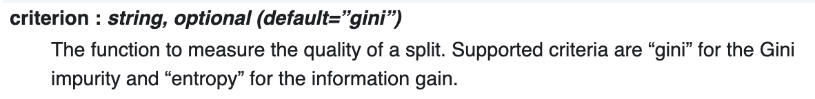
gini impurity

{\displaystyle \operatorname {I} _{G}(p)~=~1-\sum _{i=1}^{J}{p_{i}}^{2}}

information gain (entropy)

{\displaystyle \mathrm {H} (T)~=-\sum _{i=1}^{J}{p_{i}\log _{2}p_{i}}}

A single tree: hyperparameters

depth

A single tree: hyperparameters

max depth = 2

A single tree: hyperparameters

max depth = 2

PREVENTS OVERGFITTING

A single tree: hyperparameters

alternative: tree pruning

A single tree: hyperparameters

3 regression with trees

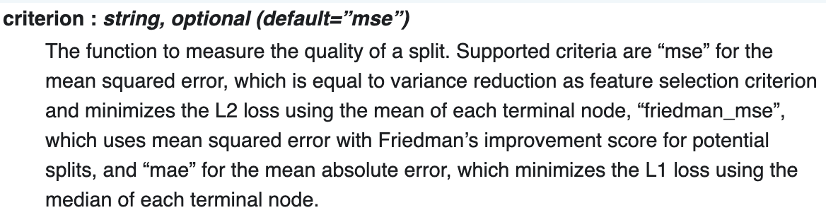
CART: Classification and Regression Trees

Trees can be used for regression

(think about it as very many small classes)

Trees can be used for regression

https://scikit-learn.org/stable/auto_examples/tree/plot_tree_regression.html

https://scikit-learn.org/stable/modules/generated/sklearn.tree.DecisionTreeRegressor.html

mean square error

A single tree: hyperparameters

mean absolute error

L_1 = \Sigma \left| y_{true} - y_{predicted}\right|

L_2= \Sigma \left( y_{true} - y_{predicted}\right)^2

4 issues with trees

variance:

different trees lead to different results

issues with trees

variance:

different trees lead to different results

why?

because calculating the criterion for every split and every mote is an untractable problem!

e.g. 2 coutinuous variables would be a problem of order

\infty^2

issues with trees

variance:

different trees lead to different results

solution

run many trees and take an "ensamble" decision!

Random Forests

Gradient Boosted Trees

a bunch of parallel trees

a series of trees

5 ensemble methods

run multiple versions of the same model with some small (stochastic or progressive) variation and learn from the emsemble of models

The decision is put together in one of two ways: bagging and boosting

Reduced variance in the decision

Reduces bias

tree ensemble methods

Gradient boosted trees: (boosting)

trees run in series (one after the other)

each tree uses different weights for the features learning the weighs from the previous tree

the last tree has the prediction

Random forest: (bagging)

trees run in parallel (independently of each other)

each tree uses a random subset of observations/features (boostrap - bagging)

class predicted by majority vote:

what class do most trees think a point belong to

tree ensemble methods

Gradient boosted trees:

Random forest:

Reading

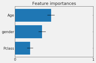
http://www.vldb.org/pvldb/vol12/p1762-paparrizos.pdf

6 feature importance

In principle CART methods are interpretable

you can measure the influence that each feature has on the decision : feature importance

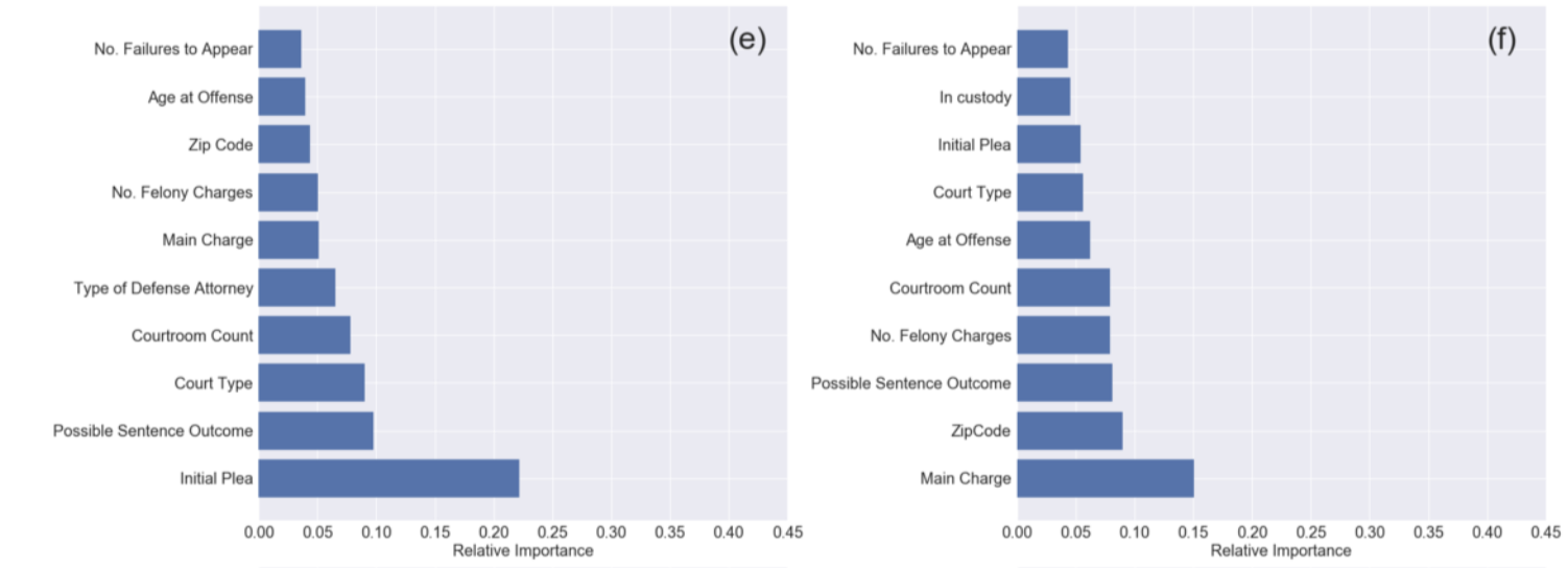
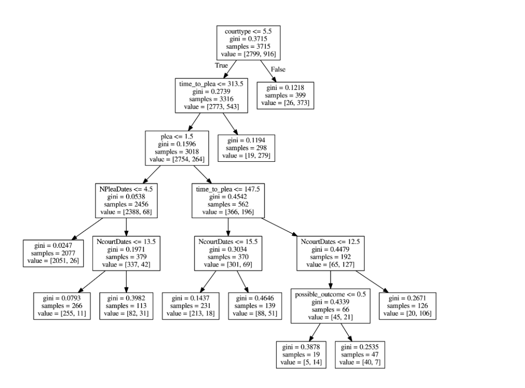
https://github.com/fedhere/DSPS/blob/master/lab9/titanictree.ipynb

https://doi.org/10.22541/au.155535549.97131926

A Data-Driven Evaluation of Delays in Criminal Prosecution

feature importance:

how soon was a feature chosen,

how many times was it used...

https://explained.ai/rf-importance/

GBT

7 encoding categorical variables

Categorical Variable

variable that can take a finite number of values.

spicies	age	weight
dog	7	32.3
bird	1	0.3
cat	3	8.1

Categorical Variable

variable that can take a finite number of values.

spicies	age	weight
dog	7	32.3
bird	1	0.3
cat	3	8.1

continuous

Categorical Variable

variable that can take a finite number of values.

spicies	age	weight
dog	7	32.3
bird	1	0.3
cat	3	8.1

continuous

ordinal

Categorical Variable

variable that can take a finite number of values.

spicies	age	weight
dog	7	32.3
bird	1	0.3
cat	3	8.1

continuous

ordinal

categorical

change categorical to (integer) numerical

one-hot encoding

spicies	age	weight
1	7	32.3
2	1	0.3
3	3	8.1

change each category to a binary

cat	bird	dog	age	weight
0	0	1	7	32.3
0	1	0	1	0.3
1	0	0	3	8.1

numerical encoding

change categorical to (integer) numerical

spicies	age	weight
1	7	32.3
2	1	0.3
3	3	8.1

change each category to a binary

implies an order that does not exist

cat	bird	dog	age	weight
0	0	1	7	32.3
0	1	0	1	0.3
1	0	0	3	8.1

one-hot encoding

numerical encoding

change categorical to (integer) numerical

spicies	age	weight
1	7	32.3
2	1	0.3
3	3	8.1

change each category to a binary

implies an order that does not exist

cat	bird	dog	age	weight
0	0	1	7	32.3
0	1	0	1	0.3
1	0	0	3	8.1

ignores covariance between features

one-hot encoding

numerical encoding

change categorical to (integer) numerical

spicies	age	weight
1	7	32.3
2	1	0.3
3	3	8.1

change each category to a binary

implies an order that does not exist

cat	bird	dog	age	weight
0	0	1	7	32.3
0	1	0	1	0.3
1	0	0	3	8.1

ignores covariance between features

one-hot encoding

numerical encoding

Definitely Preferred!

problematic if you are interested in feature importance

one-hot encoding

numerical encoding

https://github.com/fedhere/DSPS_FBianco/blob/master/labs/LocationLocationLocation.ipynb

key concepts

Machine Learning includes models that learn parameters from data

ML models have parameters learned from the data and hyperparameters assigned by the user.

Unsupervised learning:

all variables observed for all data points
learns the structure of the features space from the data
predicts a label (group of belonging) based on similarity of all features

Supervised learning:

a target feature is observed only for a subset of the data
learns target feature for data where it is not observed based on similarity of the other features
predicts a class/value for each datum without observed label

Tree methods:

partition the space one feature at a time with binary choices
prone to overfitting
can be used for regression

key concepts

single trees have high variance as the optimization has to be local

ensemble methods solve variance issue by running multiple trees and making an ensemble decision

random forest: trees run in parallel with a random subset of features

and the decision scheme is "majority" decision

gradient boosted trees: trees run in series with feature weighted learning the weights from the outcome of the previous tree. The last tree has the division

feature importance: the importance of each feature can be extracted. In presence of covariance the feature importance may be hard to interpret

key concepts

encoding categorical variables:

variables have to be encoded as numbers for computers to understand them. You can encode categorical variables with integers or floating point but you implicitly impart an order. The standard is to one-hot-encode which means creating a binary (True/False) feature (column) for each category of a categorical variables but this increases the feature space and generated covariance.

model diagnostics for classifiers: Fraction of True Positives and False Positives are the metrics to evaluate classifiers. Combinations of those numbers include Accuracy (TP/ (TP+FP)), Precision (TP/(TP+FN)), Recall ((TP+TN)/(TP+TN+FP+FN)).

ROC curve: (TP vs FP) is a holistic metric of a model. It can be used to guide the choice of hyperparameters to find the "sweet spot" for your problem

resources

http://what-when-how.com/artificial-intelligence/decision-tree- applications-for-data-modelling-artificial-intelligence/

https://www.ncbi.nlm.nih.gov/pmc/articles/PMC4466856/

https://www.youtube.com/watch?v=Trar7GZOPl8&feature=youtu.be&utm_medium=email&utm_source=intercom&utm_campaign=modular-code-event

resource on coding

resources

Distributed and parallel time series feature extraction for industrial big data applications

Maximilian Christ a , Andreas W. Kempa-Liehrb,c, Michael Fein

https://arxiv.org/pdf/1610.07717.pdf

TL;DR:

https://towardsdatascience.com/time-series-feature-extraction-for-industrial-big-data-iiot-applications-5243c84aaf0e

resources

Feature extractions from time series

https://www.twosigma.com/articles/interpretability-methods-in-machine-learning-a-brief-survey/

reading

Data Science
Interpretability Methods in Machine Learning: A Brief Survey
Insights by Two Sigma

- Download the Higgs boson data from Kaggle (programmatically within the notebook, see how in the Titanic notebook)

- Split the provided training data into a training and a test set. For each model calculate and discuss the training and test score results.

- Use a Random Forest and a Gradiend Boosted Tree Classifier model to predict the label of the particles.

- Produce a confusion matrix for each model and compare them

- Use a Random Forest and a Gradiend Boosted Tree Regressor model to predict the weight of the particles.

- Calculate the L1 and L2 metrics of each model and compare them.

- For the Random Forest classifier, select the 4 most important features (see how in the Titanic notebook) and explore the parameter space with the sklearn module sklearn.model_selection.RandomizedSearchCV for a model that uses only those features to predict the labels https://scikit-learn.org/stable/auto_examples/model_selection/plot_randomized_search.html#sphx-glr-auto-examples-model-selection-plot-randomized-search-py

- Generate an ROC curve plot for the best model and discuss it https://scikit-learn.org/stable/modules/generated/sklearn.metrics.roc_curve.html or https://scikit-learn.org/stable/auto_examples/model_selection/plot_roc_crossval.html#sphx-glr-auto-examples-model-selection-plot-roc-crossval-py

- EC and 667

---- Download the script provided in the kaggle challenge to validate your model.

---- Generate an output file as required by this script for your best model

---- Report on the result

homework

Higgs Boson Search

FDSfA 7

By federica bianco

FDSfA 7

CART methods

federica bianco

astro | data science | data for good