
federica bianco PRO
astro | data science | data for good
Neural Networks: CNN
Fall 2022 - UDel PHYS 667
dr. federica bianco
@fedhere
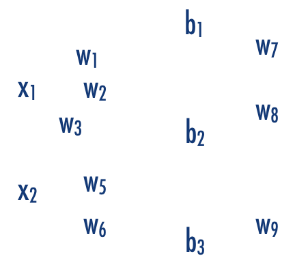
Perceptrons are linear classifiers: makes its predictions based on a linear predictor function
combining a set of weights (=parameters) with the feature vector.
.
.
.
output
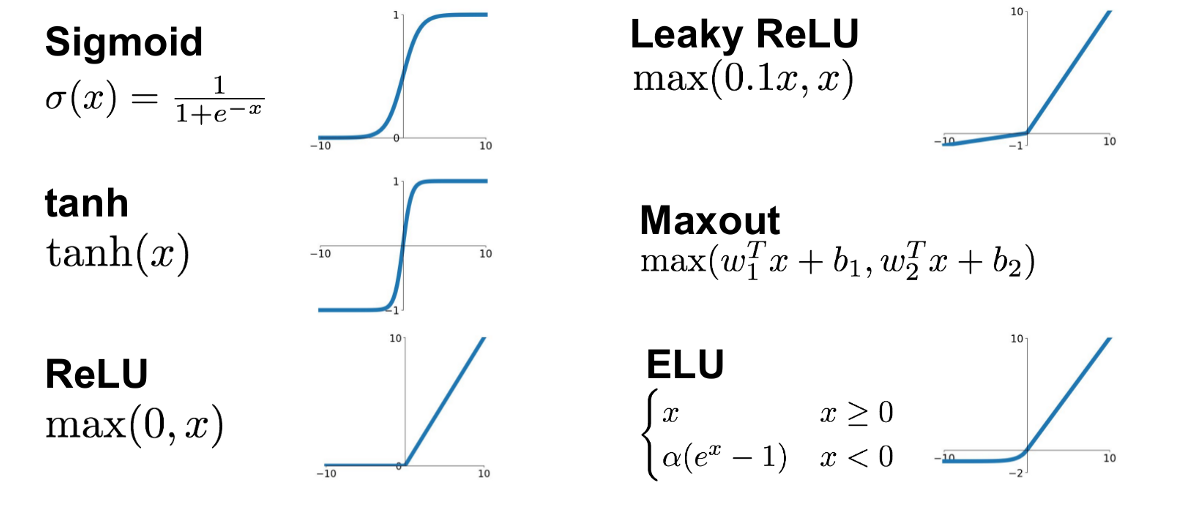
activation function
weights
bias
output
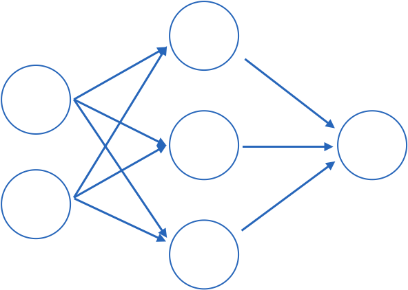
Fully connected: all nodes go to all nodes of the next layer.
input layer
hidden layer
output layer
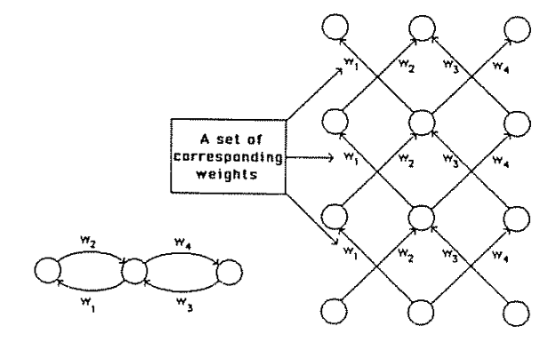
1970: multilayer perceptron architecture
output
Fully connected: all nodes go to all nodes of the next layer.
layer of perceptrons
how does linear descent look when you have a whole network structure with hundreds of weights and biases to optimize??
.
.
.
output
.
.
.
perceptron or
shallow NN
input layer
hidden layer
output layer
W4
Training models with this many parameters requires a lot of care:
- defining the metric
- choose optimization schemes
- training/validation/testing sets
But just like our simple linear regression case, the fact that small changes in the parameters leads to small changes in the output for the right activation functions.
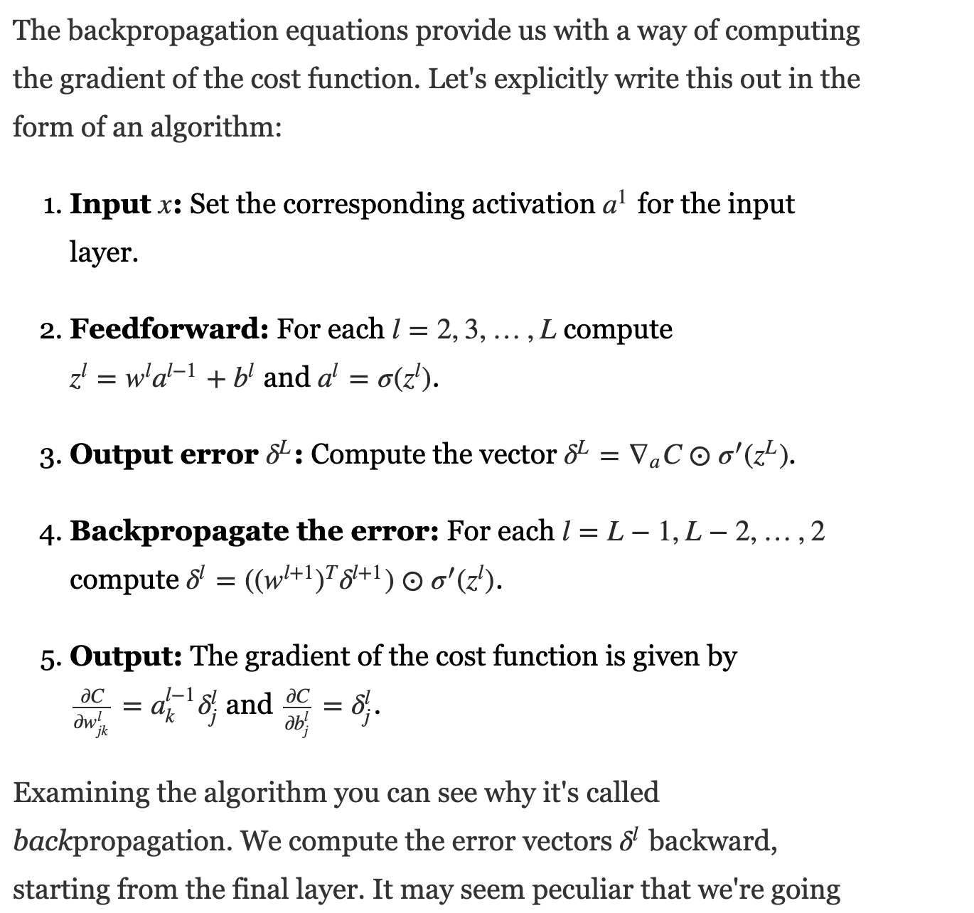
Training a DNN
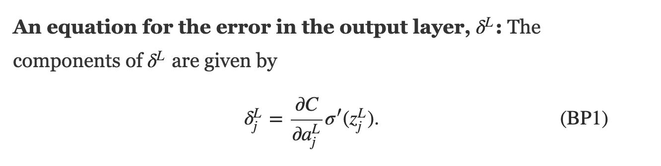
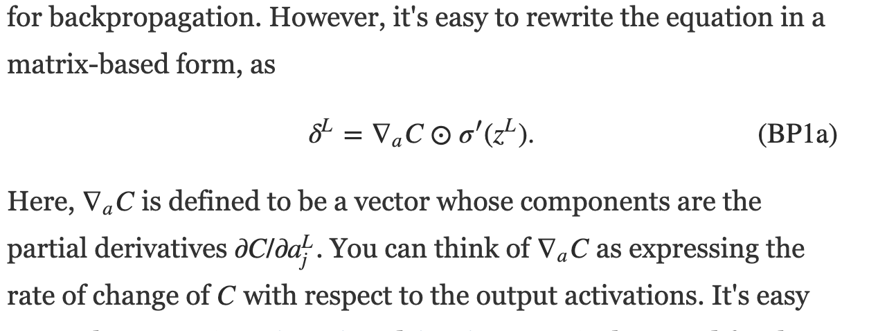
feed data forward through network and calculate cost metric
for each layer, calculate effect of small changes on next layer
define a cost function, e.g.
how does linear descent look when you have a whole network structure with hundreds of weights and biases to optimize??
think of applying just gradient to a function of a function of a function... use:
1) partial derivatives, 2) chain rule
define a cost function, e.g.
Training a DNN
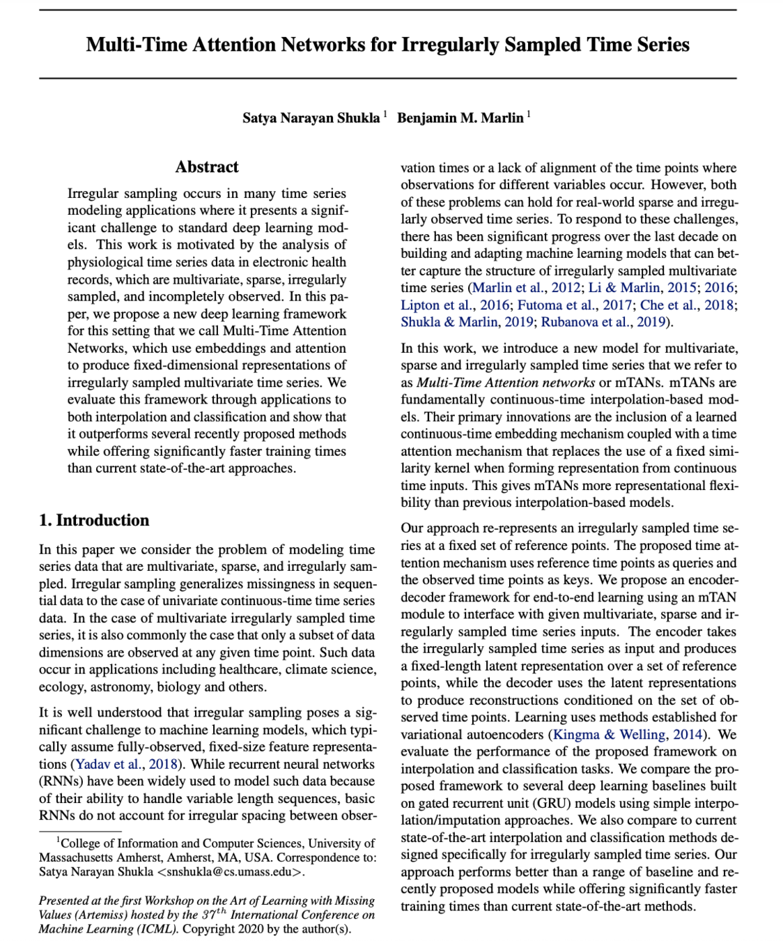
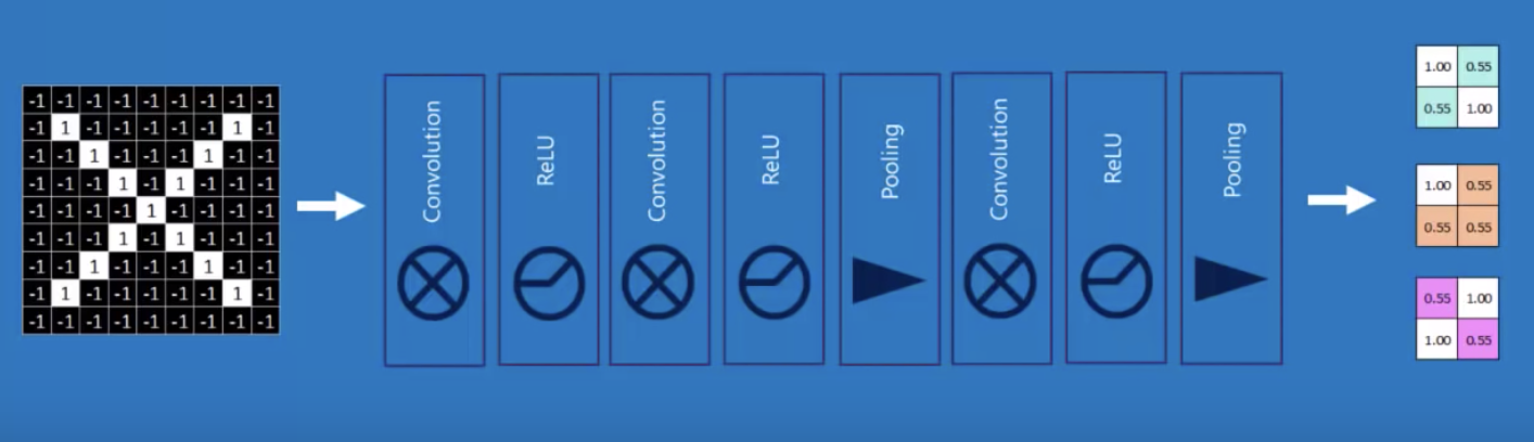
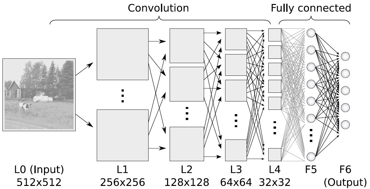
Convolutional Neural Nets
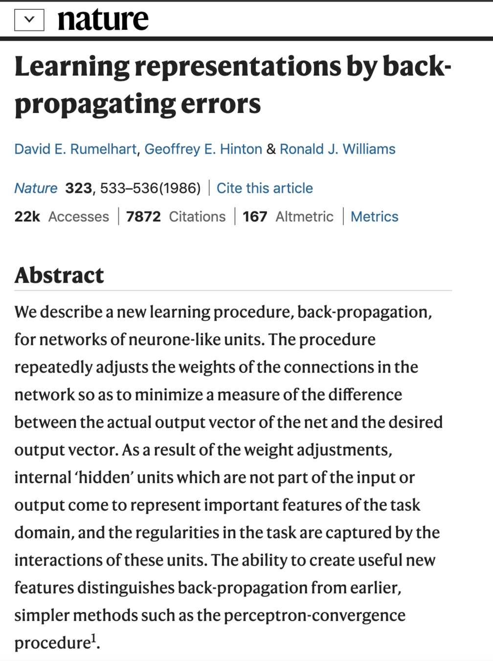
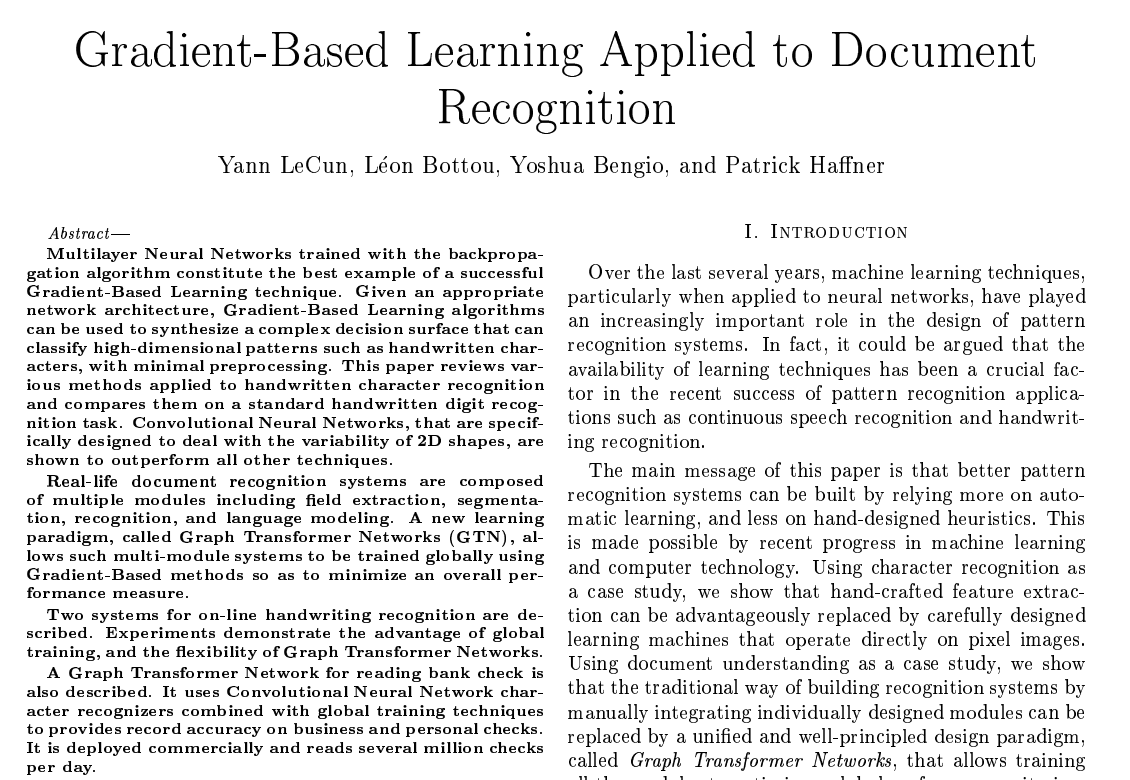
Seminal paper
Y. LeCun 1998
@akumadog
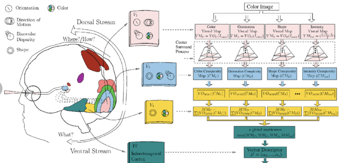
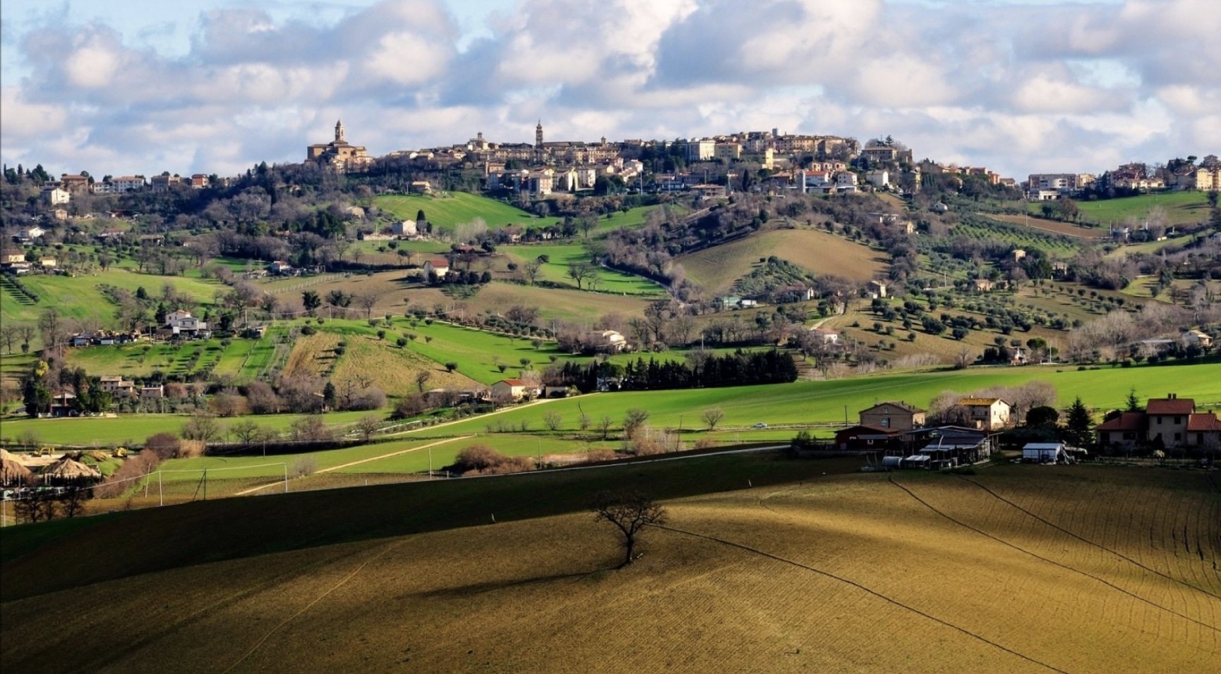
The visual cortex learns hierarchically: first detects simple features, then more complex features and ensembles of features
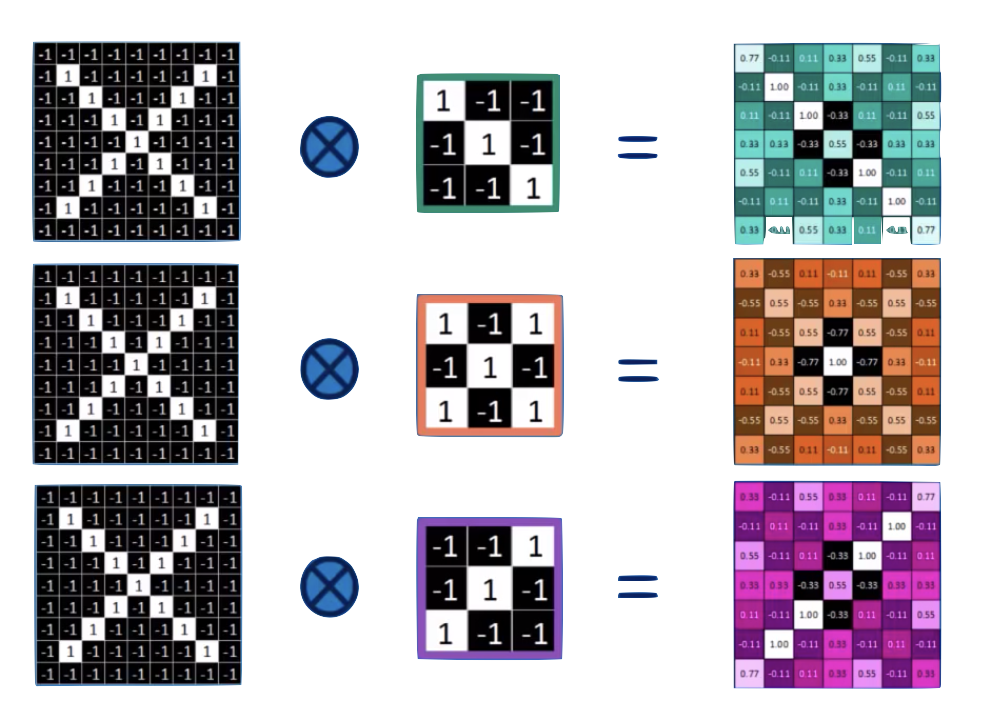
Convolution
Convolution
convolution is a mathematical operator on two functions
f and g
that produces a third function
f x g
expressing how the shape of one is modified by the other.
o
Convolution Theorem
fourier transform
two images.
| -1 | -1 | -1 | -1 | -1 |
|---|---|---|---|---|
| -1 | -1 | -1 | ||
| -1 | -1 | -1 | -1 | |
| -1 | -1 | -1 | ||
| -1 | -1 | -1 | -1 | -1 |
1
1
1
1
1
1
1
1
1
| -1 | -1 | -1 | -1 | -1 |
|---|---|---|---|---|
| -1 | -1 | -1 | -1 | -1 |
| -1 | -1 | -1 | -1 | -1 |
| -1 | -1 | -1 | -1 | -1 |
| -1 | -1 | -1 | -1 | -1 |
| 1 | -1 | -1 |
| -1 | 1 | -1 |
| -1 | -1 | 1 |
1
1
1
1
1
| -1 | -1 | -1 | -1 | -1 |
|---|---|---|---|---|
| -1 | -1 | -1 | ||
| -1 | -1 | -1 | -1 | |
| -1 | -1 | -1 | ||
| -1 | -1 | -1 | -1 | -1 |
| -1 | -1 | 1 |
| -1 | 1 | -1 |
| 1 | -1 | -1 |
feature maps
1
1
1
1
1
convolution
| -1 | -1 | -1 | -1 | -1 |
|---|---|---|---|---|
| -1 | -1 | -1 | ||
| -1 | -1 | -1 | -1 | |
| -1 | -1 | -1 | ||
| -1 | -1 | -1 | -1 | -1 |
| 1 | -1 | -1 |
| -1 | 1 | -1 |
| -1 | -1 | 1 |
1
1
1
1
1
| -1 | -1 | -1 | -1 | -1 |
|---|---|---|---|---|
| -1 | -1 | -1 | ||
| -1 | -1 | -1 | -1 | |
| -1 | -1 | -1 | ||
| -1 | -1 | -1 | -1 | -1 |
| 1 | -1 | -1 |
| -1 | 1 | -1 |
| -1 | -1 | 1 |
| 1 | -1 | -1 |
| -1 | 1 | -1 |
| -1 | -1 | 1 |
| 7 | ||
|---|---|---|
=
1
1
1
1
1
| -1 | -1 | -1 | -1 | -1 |
|---|---|---|---|---|
| -1 | -1 | -1 | ||
| -1 | -1 | -1 | -1 | |
| -1 | -1 | -1 | ||
| -1 | -1 | -1 | -1 | -1 |
| 1 | -1 | -1 |
| -1 | 1 | -1 |
| -1 | -1 | 1 |
| 1 | -1 | -1 |
| -1 | 1 | -1 |
| -1 | -1 | 1 |
| 7 | -3 | |
|---|---|---|
=
1
1
1
1
1
| -1 | -1 | -1 | -1 | -1 |
|---|---|---|---|---|
| -1 | -1 | -1 | ||
| -1 | -1 | -1 | -1 | |
| -1 | -1 | -1 | ||
| -1 | -1 | -1 | -1 | -1 |
| 1 | -1 | -1 |
| -1 | 1 | -1 |
| -1 | -1 | 1 |
| 1 | -1 | -1 |
| -1 | 1 | -1 |
| -1 | -1 | 1 |
| 7 | -3 | 3 |
|---|---|---|
=
1
1
1
1
1
| -1 | -1 | -1 | -1 | -1 |
|---|---|---|---|---|
| -1 | -1 | -1 | ||
| -1 | -1 | -1 | -1 | |
| -1 | -1 | -1 | ||
| -1 | -1 | -1 | -1 | -1 |
| 1 | -1 | -1 |
| -1 | 1 | -1 |
| -1 | -1 | 1 |
| 1 | -1 | -1 |
| -1 | 1 | -1 |
| -1 | -1 | 1 |
| 7 | -1 | 3 |
|---|---|---|
| ? | ||
=
1
1
1
1
1
| -1 | -1 | -1 | -1 | -1 |
|---|---|---|---|---|
| -1 | -1 | -1 | ||
| -1 | -1 | -1 | -1 | |
| -1 | -1 | -1 | ||
| -1 | -1 | -1 | -1 | -1 |
| 1 | -1 | -1 |
| -1 | 1 | -1 |
| -1 | -1 | 1 |
| 1 | -1 | -1 |
| -1 | 1 | -1 |
| -1 | -1 | 1 |
| 7 | -1 | 3 |
|---|---|---|
| ? | ? | |
=
1
1
1
1
1
| -1 | -1 | -1 | -1 | -1 |
|---|---|---|---|---|
| -1 | -1 | -1 | ||
| -1 | -1 | -1 | -1 | |
| -1 | -1 | -1 | ||
| -1 | -1 | -1 | -1 | -1 |
| 1 | -1 | -1 |
| -1 | 1 | -1 |
| -1 | -1 | 1 |
| 1 | -1 | -1 |
| -1 | 1 | -1 |
| -1 | -1 | 1 |
| 7 | -1 | 3 |
|---|---|---|
| ? | ? | |
=
1
1
1
1
1
| -1 | -1 | -1 | -1 | -1 |
|---|---|---|---|---|
| -1 | -1 | -1 | ||
| -1 | -1 | -1 | -1 | |
| -1 | -1 | -1 | ||
| -1 | -1 | -1 | -1 | -1 |
| 1 | -1 | -1 |
| -1 | 1 | -1 |
| -1 | -1 | 1 |
| 1 | -1 | -1 |
| -1 | 1 | -1 |
| -1 | -1 | 1 |
| 7 | -1 | 3 |
|---|---|---|
| ? | ? | |
=
1
1
1
1
1
| -1 | -1 | -1 | -1 | -1 |
|---|---|---|---|---|
| -1 | -1 | -1 | ||
| -1 | -1 | -1 | -1 | |
| -1 | -1 | -1 | ||
| -1 | -1 | -1 | -1 | -1 |
| 1 | -1 | -1 |
| -1 | 1 | -1 |
| -1 | -1 | 1 |
| 1 | -1 | -1 |
| -1 | 1 | -1 |
| -1 | -1 | 1 |
| 7 | -1 | 3 |
|---|---|---|
| ? | ? | |
=
1
1
1
1
1
| -1 | -1 | -1 | -1 | -1 |
|---|---|---|---|---|
| -1 | -1 | -1 | ||
| -1 | -1 | -1 | -1 | |
| -1 | -1 | -1 | ||
| -1 | -1 | -1 | -1 | -1 |
| 1 | -1 | -1 |
| -1 | 1 | -1 |
| -1 | -1 | 1 |
| 1 | -1 | -1 |
| -1 | 1 | -1 |
| -1 | -1 | 1 |
| 7 | -1 | 3 |
|---|---|---|
| ? | ? | |
=
1
1
1
1
1
| -1 | -1 | -1 | -1 | -1 |
|---|---|---|---|---|
| -1 | -1 | -1 | ||
| -1 | -1 | -1 | -1 | |
| -1 | -1 | -1 | ||
| -1 | -1 | -1 | -1 | -1 |
| 1 | -1 | -1 |
| -1 | 1 | -1 |
| -1 | -1 | 1 |
| 7 | -1 | 3 |
|---|---|---|
| -3 | ||
=
input layer
feature map
convolution layer
1
1
1
1
1
| -1 | -1 | -1 | -1 | -1 |
|---|---|---|---|---|
| -1 | -1 | -1 | ||
| -1 | -1 | -1 | -1 | |
| -1 | -1 | -1 | ||
| -1 | -1 | -1 | -1 | -1 |
| 1 | -1 | -1 |
| -1 | 1 | -1 |
| -1 | -1 | 1 |
| 7 | -3 | 3 |
| -3 | 5 | -3 |
| 3 | -1 | 7 |
=
input layer
feature map
convolution layer
the feature map is "richer": we went from binary to R
1
1
1
1
1
| -1 | -1 | -1 | -1 | -1 |
|---|---|---|---|---|
| -1 | -1 | -1 | ||
| -1 | -1 | -1 | -1 | |
| -1 | -1 | -1 | ||
| -1 | -1 | -1 | -1 | -1 |
| 1 | -1 | -1 |
| -1 | 1 | -1 |
| -1 | -1 | 1 |
| 7 | -3 | 3 |
| -3 | 5 | -3 |
| 3 | -1 | 7 |
=
input layer
feature map
convolution layer
the feature map is "richer": we went from binary to R
and it is reminiscent of the original layer
7
5
7
Convolve with different feature: each neuron is 1 feature
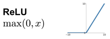
ReLu
| 7 | -3 | 3 |
| -3 | 5 | -3 |
| 3 | -1 | 7 |
7
5
7
ReLu: normalization that replaces negative values with 0's
| 7 | -3 | 3 |
| -3 | 5 | -3 |
| 3 | -1 | 7 |
7
5
7
ReLu: normalization that replaces negative values with 0's
| 7 | 0 | 3 |
| 0 | 5 | 0 |
| 3 | 0 | 7 |
7
5
7
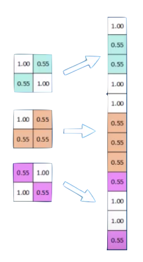
Max-Pool
MaxPooling: reduce image size, generalizes result
| 7 | 0 | 3 |
| 0 | 5 | 0 |
| 0 | 0 | 7 |
7
5
7
MaxPooling: reduce image size, generalizes result
| 7 | 0 | 3 |
| 0 | 5 | 0 |
| 3 | 0 | 7 |
7
5
7
2x2 Max Poll
| 7 | 5 |
MaxPooling: reduce image size, generalizes result
| 7 | 0 | 3 |
| 0 | 5 | 0 |
| 3 | 0 | 7 |
7
5
7
2x2 Max Poll
| 7 | 5 |
| 5 |
MaxPooling: reduce image size, generalizes result
| 7 | 0 | 3 |
| 0 | 5 | 0 |
| 3 | 0 | 7 |
7
5
7
2x2 Max Poll
| 7 | 5 |
| 5 | 7 |
MaxPooling: reduce image size & generalizes result
By reducing the size and picking the maximum of a sub-region we make the network less sensitive to specific details
x
O
last hidden layer
output layer
Stack multiple convolution layers
Minibatch
&
Dropout
Split your training set into many smaller subsets and train on each small set separately
Dropout
Artificially remove some neurons for different minibatches to avoid overfitting
output
EITHER:
we take a look at DeepDream
OR
we take a look at a convolutional NN code
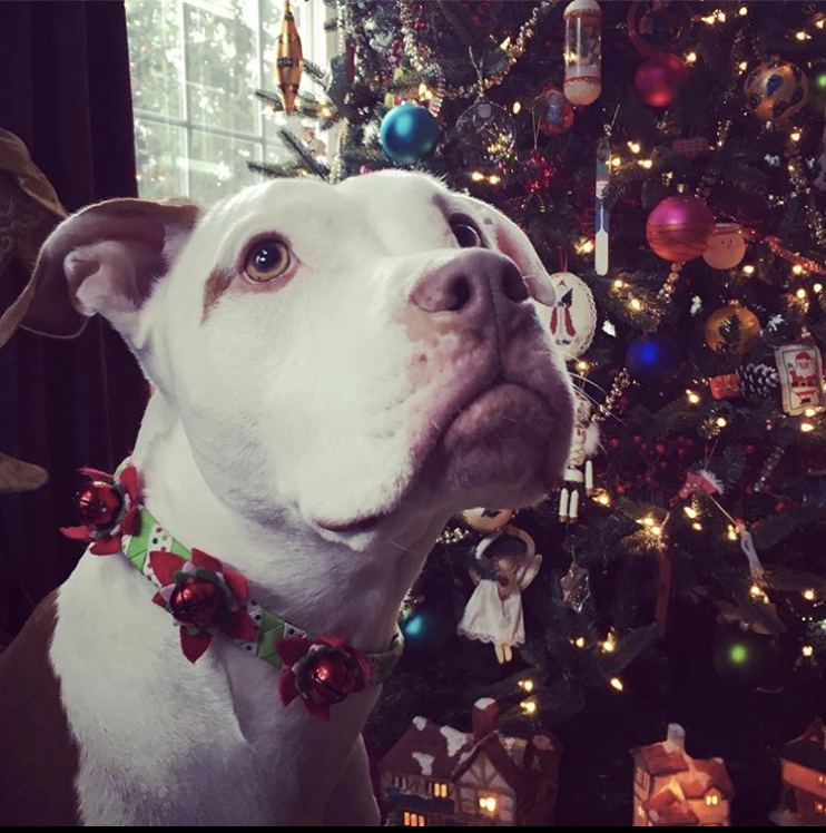
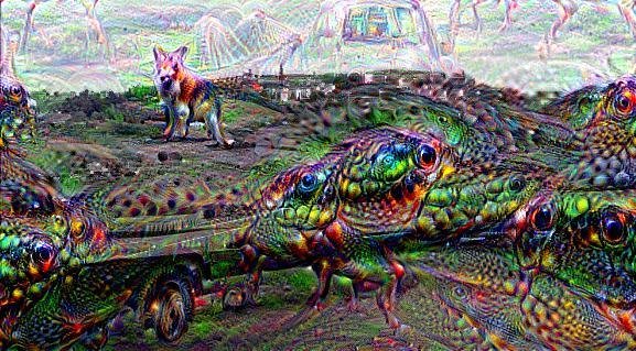
Deep Dream (DD) is a google software, a pre-trained NN (originally created on the Cafe architecture, now imported on many other platforms including tensorflow).
The high level idea relies on training a convolutional NN to recognize common objects, e.g. dogs, cats, cars, in images. As the network learns to recognize those objects is developes its layers to pick out "features" of the NN, like lines at a cetrain orientations, circles, etc.
The DD software runs this NN on an image you give it, and it loops on some layers, thus "manifesting" the things it knows how to recognize in the image.
CNN
Object detection
Naive model: we took different region of the image and measured the probability of presence of the object in that region
Object detection
Problem: we had to search the whole image which is time consuming, we could only find 1 kind of object at 1 scale
CNN
YOLO and R-CNN
Object detection
What if you do not know what is in the mage?
Final Dense layer has undefined size (one per kind of object in the region)
Objects can have different scale or axis ration: how many regions can you search before the problem blows up computationally??
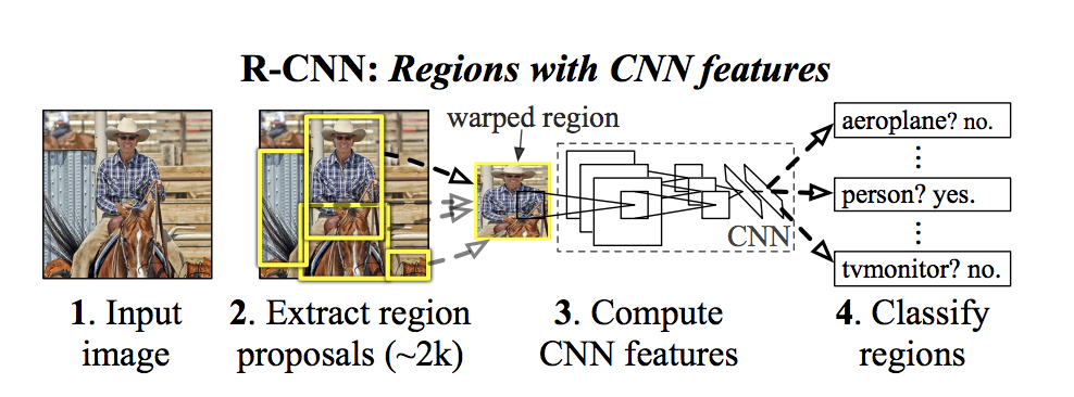
R-CNN
Extract 2000 regions from the image "region proposals."
Feature Extraction CNN produces a 4096-dimensional feature vector in an output dense layer
SVM classify the presence of the object within that candidate region proposal.
1. Generate initial sub-segmentation, we generate many candidate     regions
2. Use greedy algorithm to recursively combine similar regions into larger ones
3. Use the generated regions to produce the final candidate region proposals
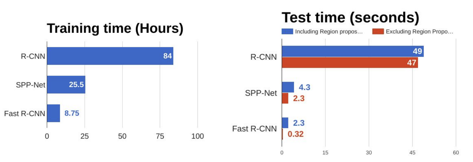
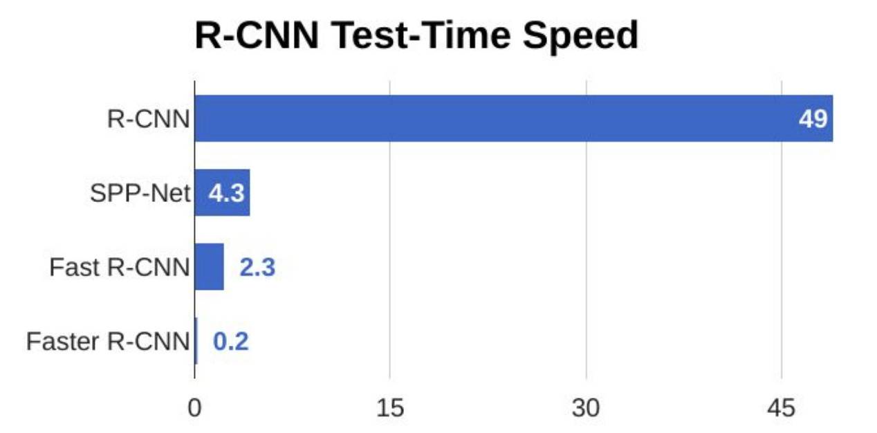
TOO SLOW (47 sec to test 1 image)
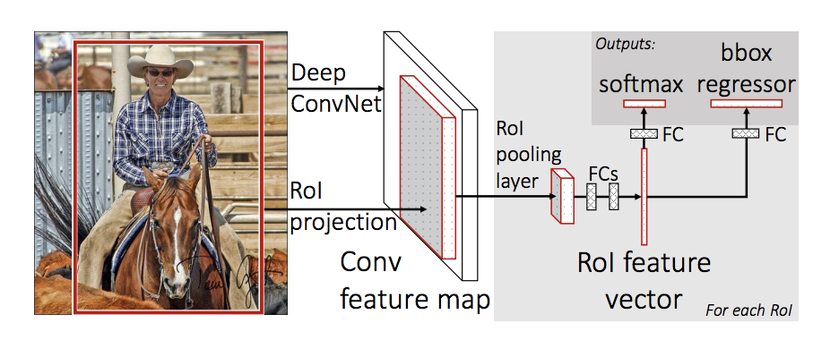
Fast R-CNN
Use a CNN to generate convolutional feature maps
Use Selective Search Algorithm to tdentify the RPs and warp them into squares
Using an RoI pooling layer to reshape them into a fixed size so that it can be fed into a fully connected layer - predict box offset
Softmax layer to predict the class of the proposed
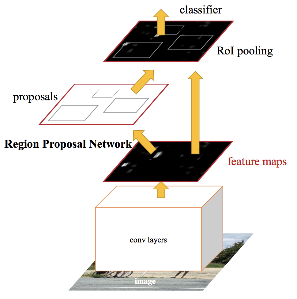
Faster R-CNN
Use a CNN to generate convolutional feature maps
Use CNN to predict RPs and warp them into squares
Using an RoI pooling layer to reshape them into a fixed size so that it can be fed into a fully connected layer - predict box offset
Softmax layer to predict the class of the proposed
Faster R-CNN
Ren et al. 2015
Use a CNN to generate convolutional feature maps
Use CNN to predict RPs and warp them into squares
Using an RoI pooling layer to reshape them into a fixed size so that it can be fed into a fully connected layer - predict box offset
Softmax layer to predict the class of the proposed
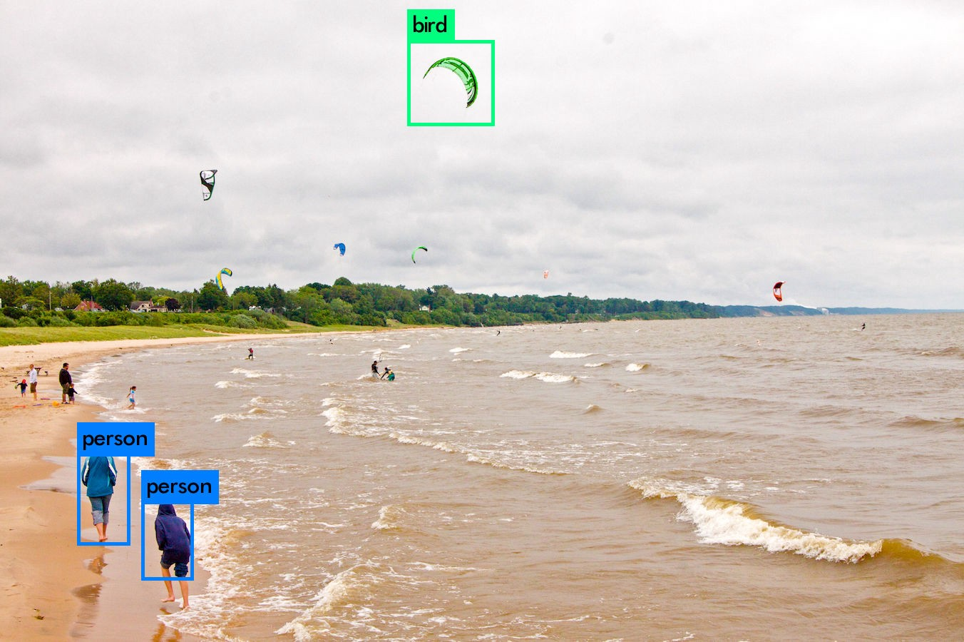
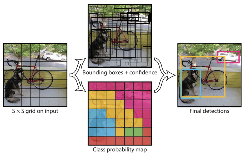
Yolo
What if you looked at the whole image instead of RoIs in the image??
Split an image into a SxS grid
For each grid cell predicts B bounding boxes, confidence for those boxes, and C class probabilities.
CNN outputs probability that BB has an object (+ offset)
High prob BBs are classified
Yolo
What if you looked at the whole image instead of RoIs in the image??
Split an image into a SxS grid
For each grid cell predicts B bounding boxes, confidence for those boxes, and C class probabilities.
CNN outputs probability that BB has an object (+ offset)
High prob BBs are classified
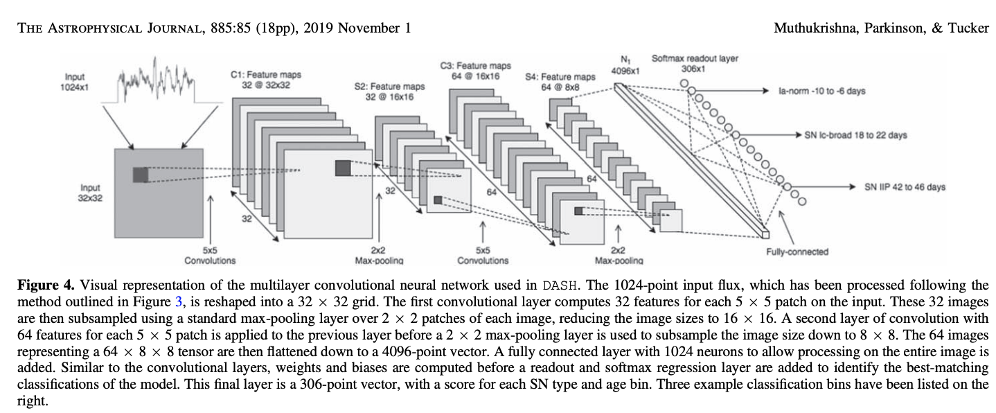
https://arxiv.org/abs/1902.01466
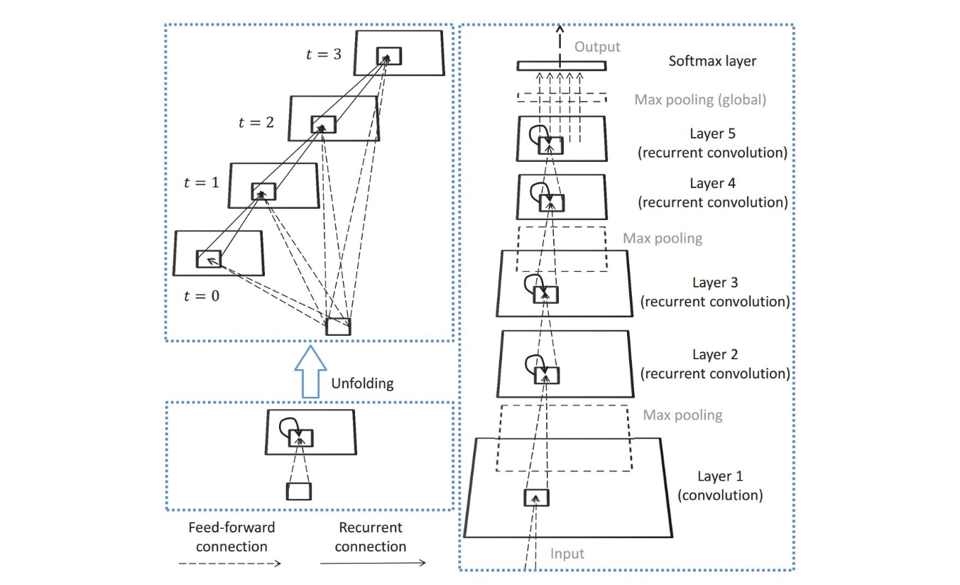
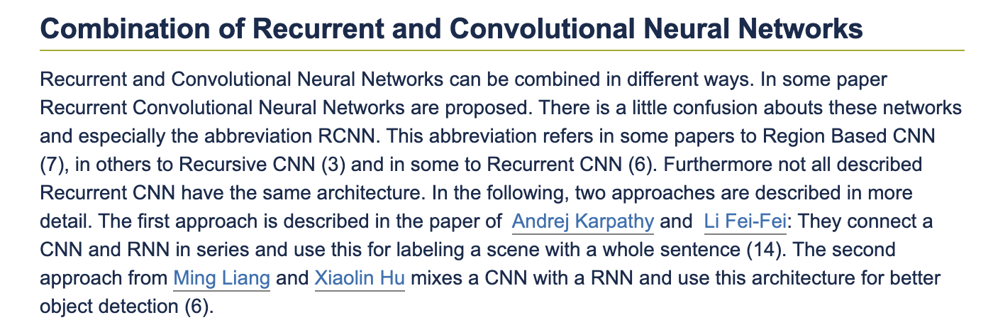
CNNs for image sequences
Recurrent CNN
Architecture components: neurons, activation function
Single layer NN: perceptrons
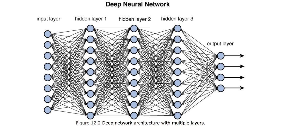
Deep NN:
Convolutional NN
Training an NN:
My proposal is based upon an asymmetry between verifiability and falsifiability; an asymmetry which results from the logical form of universal statements. For these are never derivable from singular statements, but can be contradicted by singular statements.
—Karl Popper, The Logic of Scientific Discovery
the demarcation problem:
what is science? what is not?
the demarcation problem
in Bayesian context
The probability that a belief is true given new evidence equals the probability that the belief is true regardless of that evidence times the probability that the evidence is true given that the belief is true divided by the probability that the evidence is true regardless of whether the belief is true.
- Thomas Bayes Essay towards solving a Problem in the Doctrine of Chances (1763)
Principle of Parsimony
Between two models with the same explanatory power choose the one with fewer parameters
Likelihood Ration Test | AIC | BIC | Kullback Divergence
Reproducible research in practice:
using the code and raw data provided by the analyst.
Claerbout, J. 1990,
Active Documents and Reproducible Results, Stanford Exploration Project Report, 67, 139
Reproducible research means:
the ability of a researcher to duplicate the results of a prior study using the same materials as were used by the original investigator. That is, a second researcher might use the same raw data to build the same analysis files and implement the same statistical analysis in an attempt to yield the same results.
all numbers in a data analysis can be recalculated exactly (down to stochastic variables!)
parameters (-0.1, 0.9)
support
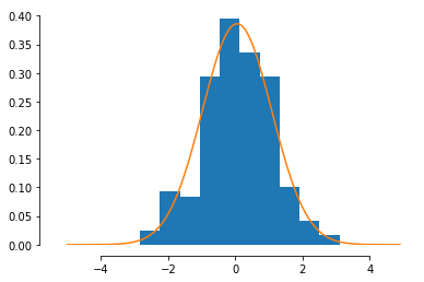
normal or Gaussian
continuous support
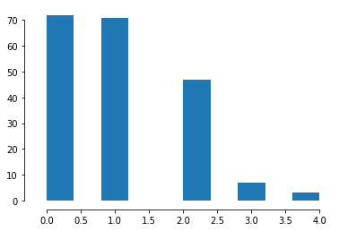
Poisson
discrete support
parameters (lambda=1)
a distribution’s moments summarize its properties:
central tendency: mean (n=1), median, mode
spread: standard deviation/variance (n=2), quartiles range
symmetry: skewness (n=3)
cuspiness: kurtosis (n=4)
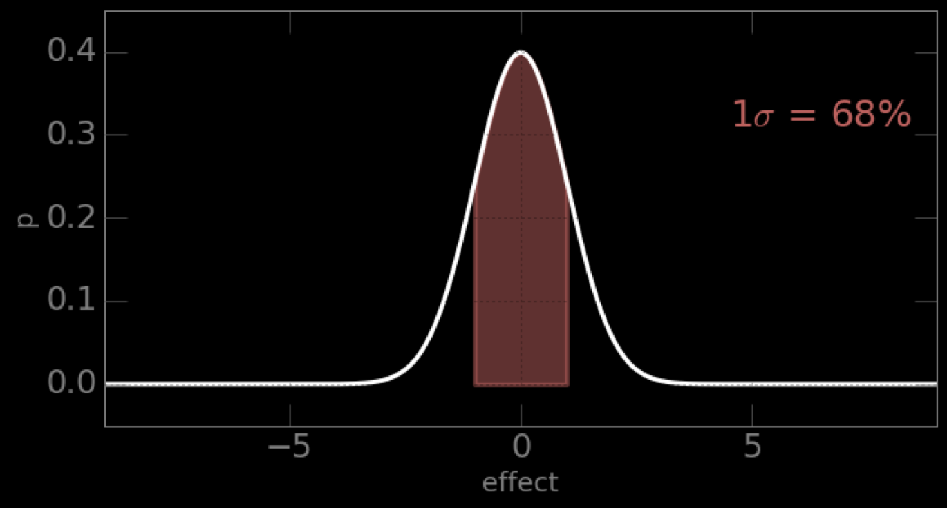
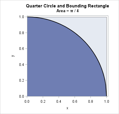
Why am I bothering with areas? - Expectation values are related to areas
The ratio of the area of the circle to the area of the square is π / 4.
Calculate Pi
https://www.jstor.org/stable/2686489?seq=1
https://github.com/fedhere/DSPS_FBianco/tree/master/montecarlo
choose a starting point in the parameter space: current = θ0 = (m0,b0)
WHILE convergence criterion is met:
calculate the current posterior pcurr = P(D|θ0,f)
//proposal
choose a new set of parameters new = θnew = (mnew,bnew)
calculate the proposed posterior pnew = P(D|θnew,f)
IF pnew/pcurr > 1:
current = new
ELSE:
//probabilistic step: accept with probability pnew/pcurr
draw a random number r ૯U[0,1]
IF r > pnew/pcurr >:
current = new
ELSE:
pass // do nothing
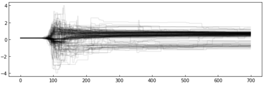
step
feature value
choose a starting point in the parameter space: current = θ0 = (m0,b0)
WHILE convergence criterion is met:
calculate the current posterior pcurr = P(D|θ0,f)
//proposal
choose a new set of parameters new = θnew = (mnew,bnew)
calculate the proposed posterior pnew = P(D|θnew,f)
IF pnew/pcurr > 1:
current = new
ELSE:
//probabilistic step: accept with probability pnew/pcurr
draw a random number r ૯U[0,1]
IF pnew/pcurr > r:
current = new
ELSE:
pass // do nothing
Examples of how to choose the next point
affine invariant : EMCEE package
classification
prediction
feature selection
supervised learning
understanding structure
organizing/compressing data
anomaly detection dimensionality reduction
unsupervised learning
clustering
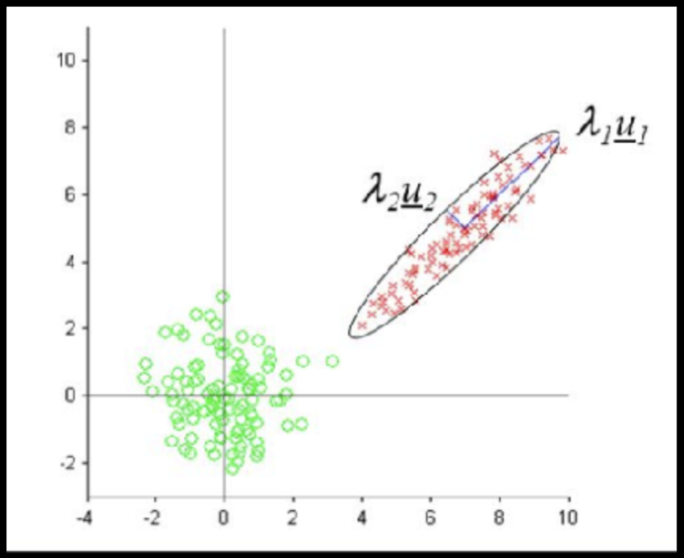
PCA
Apriori
k-Nearest Neighbors
Regression
Support Vector Machines
Classification/Regression Trees
Neural networks
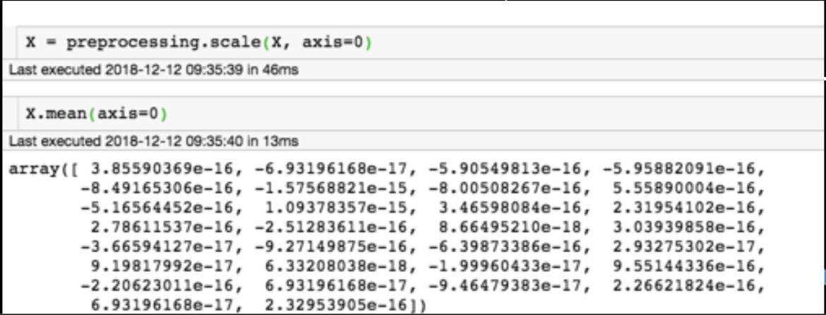
Generic preprocessing
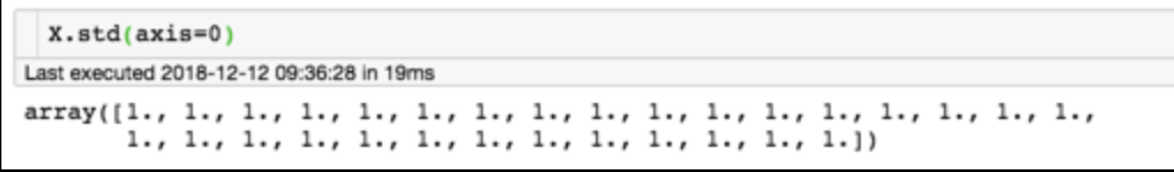
for each feature: divide by standard deviation and subtract mean
mean of each feature should be 0, standard deviation of each feature should be 1
change categorical to (integer) numerical
| spicies | age | weight |
|---|---|---|
| 1 | 7 | 32.3 |
| 2 | 1 | 0.3 |
| 3 | 3 | 8.1 |
change each category to a binary
| cat | bird | dog | age | weight |
|---|---|---|---|---|
| 0 | 0 | 1 | 7 | 32.3 |
| 0 | 1 | 0 | 1 | 0.3 |
| 1 | 0 | 0 | 3 | 8.1 |
LR = _____________________________
True Negative
False Negative
| H0 is True | H0 is False | |
|---|---|---|
| H0 is falsified | Type I Error False Positive |
True Positive |
|
H0 is not falsified |
True Negative | Type II Error False Negative |
GOOD
BAD
what is the simplest classifier you can build for this dataset ?
what is the accuracy?
x
y
If your dataset is imbalanced (more of one class than the other)
your model will learn that it is better to guess the most common class
this will contaminate the prediction
Partition (unsupervised)
Classification (supervised)
Regression (supervised)
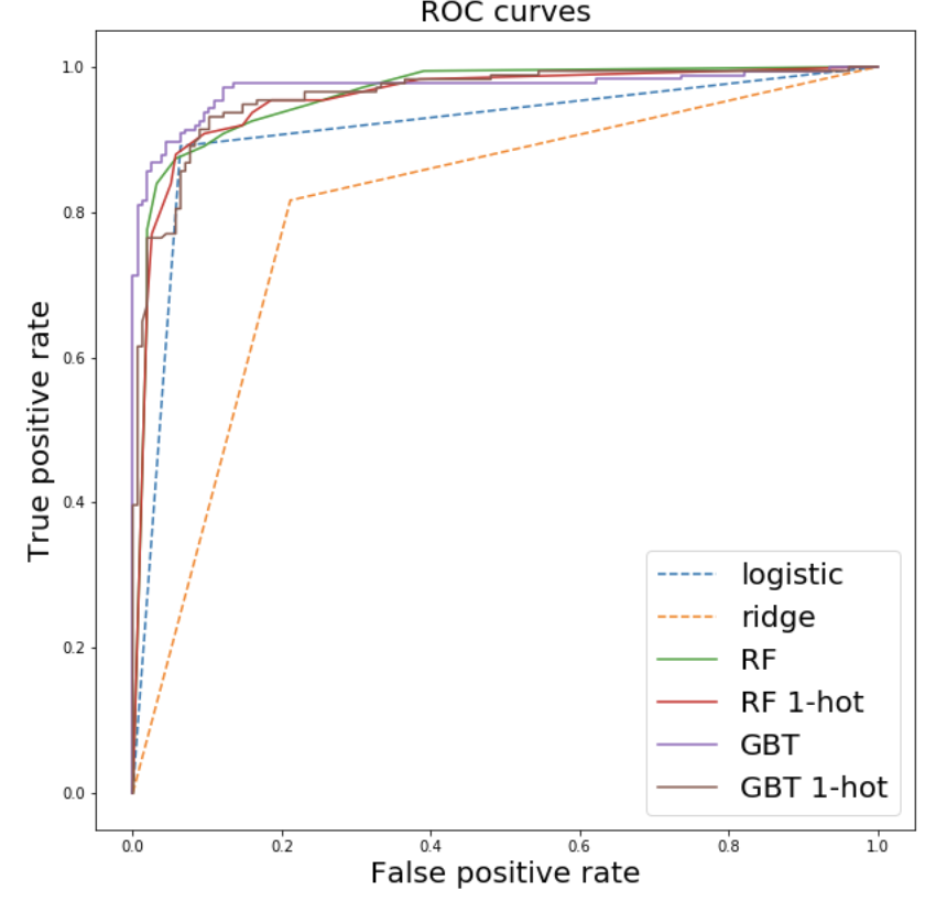
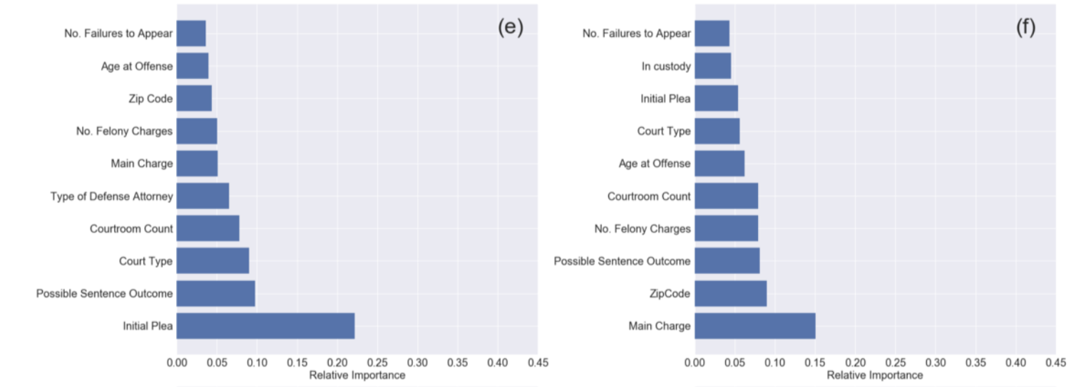
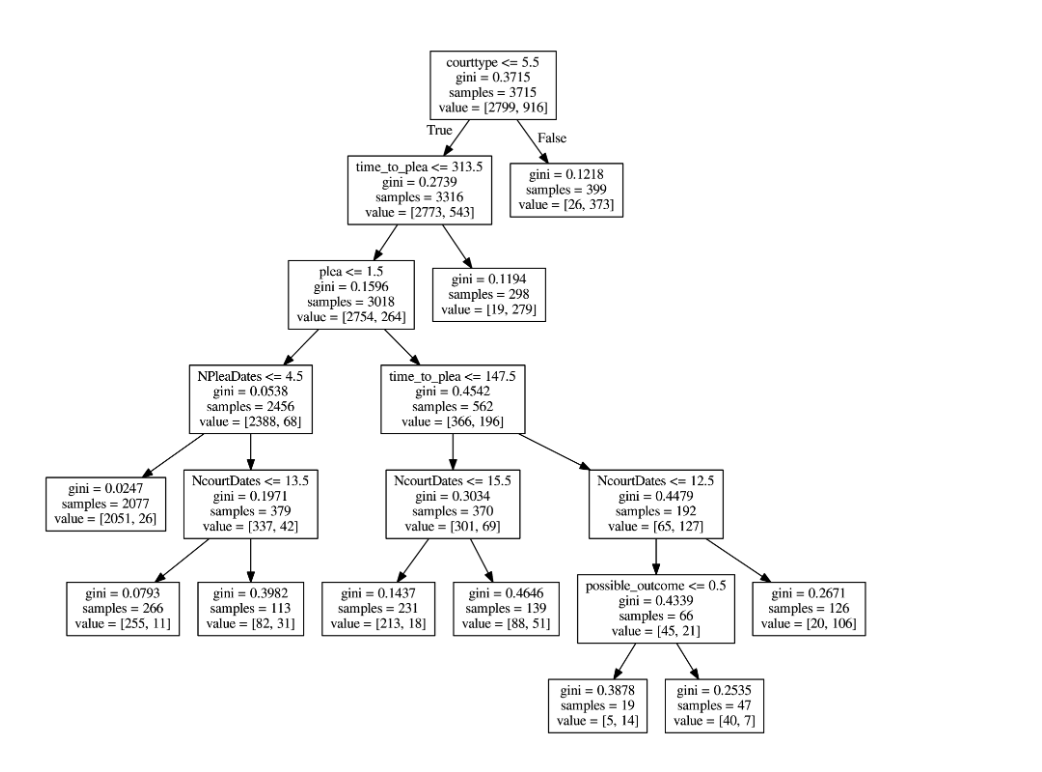
A Data-Driven Evaluation of Delays in Criminal Prosecution
feature importance:
how soon was a feature chosen,
how many times was it used...
RF
GBT
It can be shown that the optimal parameters for a line fit to data without uncertainties is:
from sklearn.linear_model import LinearRegression
lr = LinearRegression()

X = np.c_[np.ones(len(x)), x]
lr.fit(X, y)
lr.coef_, lr.intercept_
We can let sklearn solve the equation for us:
2x1
2xN Nx2 2xN Nx1
x = np.sort(10 * np.random.rand(N))
y = x * m_true + b_true
yerr = 0.1 + 0.5 * np.random.rand(N)
y += np.abs(f_true * y) * np.random.randn(N) + yerr * np.random.randn(N)

X = np.c_[np.ones(len(x)), x]
theta_best = np.linalg.inv(X.T.dot(X)).dot(X.T).dot(y)
Neural Network and Deep Learning an excellent and free book on NN and DL http://neuralnetworksanddeeplearning.com/index.html
History of NN https://cs.stanford.edu/people/eroberts/courses/soco/projects/neural-networks/History/history2.html
Raissi et al. Physics Informed Deep Learning (Part I): Data-driven Solutions of Nonlinear Partial Differential Equations. arXiv 1711.10561
Raissi et al. Physics Informed Deep Learning (Part II): Data-driven Discovery of Nonlinear Partial Differential Equations. arXiv 1711.10566
Raissi et al. Physics-informed neural networks: A deep learning framework for solving forward and inverse problems involving nonlinear partial differential equations. J. Comp. Phys. 378 pp. 686-707 DOI: 10.1016/j.jcp.2018.10.045
By federica bianco
convolutional neural networks


