Z-mappings
for mathematicians
Flavien Léger

Joint work with Alfred Galichon (NYU)
Nonvariational, nonlinear equations discrete and continuous
Common structure to problems in network flows, optimal transport, optimal control, interface dynamics, submodular functions...
Dates back to Rheinboldt ('70s)
Ideal to prove comparison principles
Persists through regularization and continuous ↔ discrete
Prelude
Natural algorithm: Jacobi
Outline
1. Z-mappings
2. M-mappings
3. The Jacobi algorithm
4. Examples
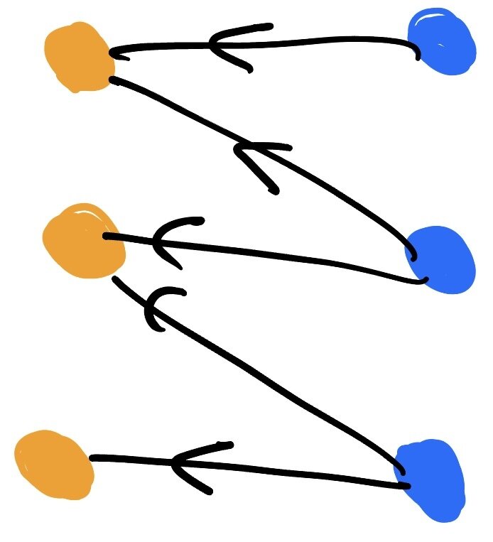
1. Z-mapping
\(Q\) is a Z-mapping if for all \(u,\tilde u\), for all \(x\),
D E F I N I T I O N
Want to solve equations of the form
$$Q(u) = 0,$$
\(u\colon X\to\mathbb{R}\), \(X\) finite or \(X\subseteq\mathbb{R}^d\)
\(Q\colon \mathbb{R}^X\to\mathbb{R}^X\)

Toy example: \(Q_i(u)=2u_i-u_{i+1}-u_{i-1}.\)
Examples
Square matrix \(A\), solve
\[Au=f\]
Let \(Q(u) = Au-f\). Then
\[Q\text{ is a Z-mapping }\quad\iff\quad a_{ij}\le 0 \text{ for all }i\neq j.\]
Z-matrix

On a network \((X,A)\),
\[-\mathrm{div} M(u)=f\]
\(M\colon\mathbb{R}^X\to\mathbb{R}^A\) "flow mapping" such that:
\(M_{xy}(u)\) increasing in \(u_y\) decreasing in \(u_x\).
Ex: \(M_{xy}(u)=u_y-u_x\),
\(M_{xy}(u)=e^{u_y-u_x}\)
Examples
\[\partial_tu=-Q(u)\]
If \(Q\) is a Z-mapping then so is the spacetime mapping
$$\hat Q_{t,x}(u)\coloneqq \frac{u_{t,x}-u_{t-1,x}}{\tau}+ Q_x(u_t)$$
\(Q(u)\coloneqq u - T(u)\) is a Z-mapping.
(Shortest path, stochastic shortest path, Markov Decision Process)

Dynamic programming principle:
\[u(x)=\min_{y}c(x,y)+u(y)\eqqcolon T(u)\]
(Eikonal equation, Hamilton–Jacobi Bellman, viscosity solutions)
2. M-mappings
A Z-mapping \(Q\) is an M-mapping if it satisfies a comparison principle
$$Q(u)\leq Q(\tilde u)\implies u\leq \tilde u$$
D E F I N I T I O N
\(Q(u)=f,\,Q(\tilde u)=\tilde f \text{ with } f\leq \tilde f \implies u\leq \tilde u\)
Uniqueness of \(Q(u)=f\)
Maximum principle
Strong comparison principle: if \(V\) is a strongly connected component of an M-mapping \(Q\) then
$$Q(u)\leq Q(\tilde u)\implies u=\tilde u \text{ or } u <\tilde u \text{ on } V.$$
Suppose that a Z-mapping \(Q\) satisfies: for all \(V\subseteq X\),
\[\left\{\begin{aligned}u&<\tilde u \text{ on } V\\u&=\tilde u \text{ on }X\setminus V\end{aligned}\right.\implies\sum_{x\in V} Q_x(u)<\sum_{x\in V} Q_x(\tilde u)\]
Then \(Q\) is an M-mapping.
T H E O R E M
Berry, Gandhi, Haile '2013; Chen, Choo, Galichon, Weber '2021
Example: \(Q(u)=-\operatorname{div}(a(x,u)\nabla u)-f,\quad a(x,u)\geq c_0>0\)
\[\int_V Q(u)dx=\int_{\partial V} a(x,u)\langle\nabla u,- n\rangle\]
Works for quasilinear PDEs, Monge–Ampère, semi-discrete optimal transport, entropic transport...
Proving a comparison principle
Basic idea: combine the Z-property and “some isotonicity”
3. The Jacobi algorithm
D E F I N I T I O N
The Jacobi transform \(J\colon \mathbb{R}^X\to\mathbb{R}^X\) is defined by
\[Q_x(J_x(u),u_{-x})=0.\]
Jacobi algorithm
\[u_{n+1} = J(u_n)\]
A L G O R I T H M
“coordinate update”
Also related: Gauss–Seidel
Properties of Jacobi
Let \(Q\) be a continuous Z-mapping.
1. If \(Q(u_n)\le 0\) then
\[Q(u_{n+1})\le 0 \quad\text{and}\quad u_n\leq u_{n+1}\]
2. \[u_n\le \tilde u_n \implies u_{n+1}\leq \tilde{u}_{n+1}\]
P R O P O S I T I O N
1: Useful for algorithm or showing existence of solutions
"method of subsolutions", "Perron's method"...
2: Useful when sandwich \(v_0\le u_0\le w_0\), then
\[v_n\le u_n\le w_n\]
Rheinbolt ’70
Optimal transport (continuous/discrete/semi-discret/entropic), generated Jacobian equations
\[S_u(y)\coloneqq \argmax_x u(x)-c(x,y)\]
⏵ Discrete: \(Q\) is discontinuous \(\to\) need regularization.
Real auction, or replace min by softmin: Entropic OT.
\[S_{u\#}\nu=\mu\]
\(Q(u) = S_{u\#}\nu\) is a Z-mapping
⏵ Algorithm: Jacobi = Bertsekas' (naive) auction algorithm
4. Examples
⏵ Monge–Ampère has a comparison principle
⏵ Jacobi = Sinkhorn

Mean curvature motion
mean curvature motion = \(L^2\) gradient flow of
\[P(u)=\frac12\int_{\mathbb{R}^d} \lvert\nabla u\rvert\,dx\]
(\(u=1_K\)). Heat content:
\[P_\varepsilon(u)=-\frac{1}{\varepsilon}\iint G_\varepsilon(x-y) u(x) (1-u(y))\,dxdy + \int \chi(u(x))\,dx\]
submodular, nonconvex
\(Q(u)=DP(u)\) is a Z-mapping.
⏵ Jacobi = MBO
(Merriman–Bence–Osher ’92)
Thank you!
(Dauphine 2023-12-20) Z-mappings
By Flavien Léger
(Dauphine 2023-12-20) Z-mappings
- 475


