Contact-Implicit MPC:
Methods analysis and comparison
Grey Sarmiento
Ph.D. Qualifying Exam

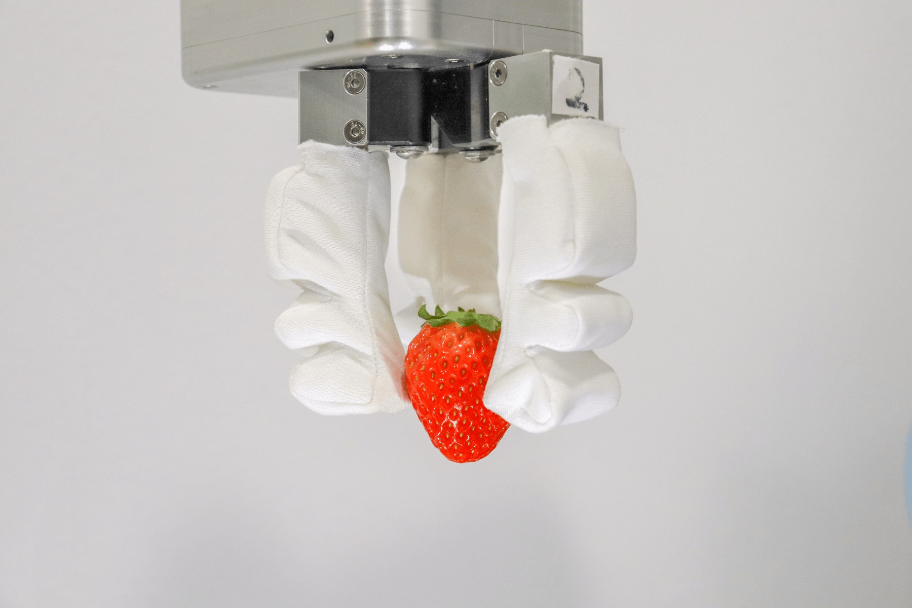
Making contact with the environment is critical for many robotic tasks.
Contact planning and control decides how and when the robot should contact the world.
Example tasks:
- Flip a block onto a different face.
- Walk up a rugged hill.
- Slide a tray off a table.
- Use the guardrail to catch yourself if you fall.
Ask the questions:
- What block face(s) should I touch?
- Where should I step and with what gait?
- Which way should I push the tray? How fast should I move?
- When should I reach out to the rail?
Problem: Contact causes discontinuous dynamics and nonconvex constraints.
\lambda_z = 0
\varphi = +\varepsilon
\varphi
F_z
F_x
Problem: Contact causes discontinuous dynamics and nonconvex constraints.
\lambda_z >> 0
\varphi = -\varepsilon
\lambda_z
F_z
Problem: Contact causes discontinuous dynamics and nonconvex constraints.
\mu F_{z}-\Vert F_ x\Vert = +\varepsilon
v_{\textrm{robot,x}}> 0
F_z
F_x
Problem: Contact causes discontinuous dynamics and nonconvex constraints.
v
\varphi = 0
\mu F_{z}-\Vert F_ x\Vert=0
Problem: Contact causes discontinuous dynamics and nonconvex constraints.
Contact dynamics are discontinuous at contact boundaries.
Task success is brittle to error or misestimation of force, friction, position, distance, and velocity
Deciding when to make and break contact is difficult if dynamics are used in the contact planner
Many important tasks require navigating many options for contact and contact mode in order to be successful, which can be computationally expensive
The full contact planning problem becomes very hard to solve.
To handle this, contact planners and controllers make different approximations of the true problem.
Our challenge: Compare these different methods and understand when each method works, and when/why they fail
- Decrease the number of contact modes being considered
- Modify the dynamics to be continuous, differentiable, and/or convex
- Avoid modeling contact directly
- Break the problem into convex segments and then enforce their agreement
- Related work on contact
- Preliminaries and background
- Contact-implicit literature review
- Overview of methods analyzed
- Experiments and Discussion
- Future Work
Presentation Outline
Related Work
1
- Related work on contact
- Preliminaries and background
- Contact-implicit literature review
- Overview of methods analyzed
- Experiments and Discussion
- Future Work
- Related work on contact
Low-level methods for contact uncertainty
- Passive compliance (such as mechanical compliance and soft robots) and active compliance (such as impedance control) can help with contact instability and contact error
- still requires a higher-level controller that decides the contact trajectory
Methods for planning over contact
Explicit and Hierarchical Contact Sequences
Idea: Solve for the optimal trajectory in each contact mode and use a pre-specified schedule or higher-level planner for contact sequence
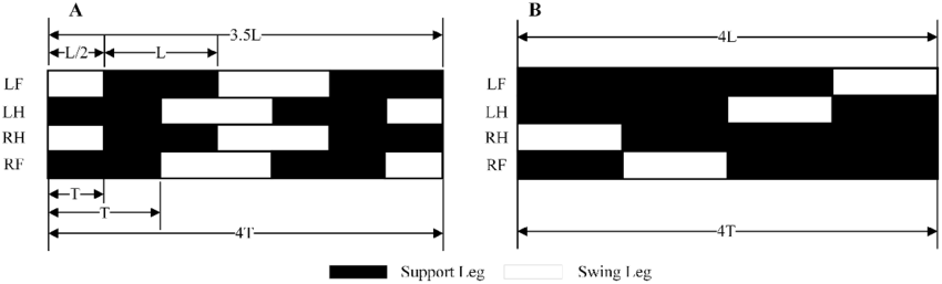
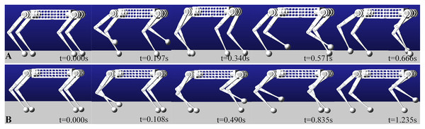
W. Yan, Y. Pan, J. Che, J. Yu, and Z. Han, “Whole-body kinematic and dynamic modeling for quadruped robot under different gaits and mechanism topologies,” PeerJ Computer Science, vol. 7, p. e821, 2021
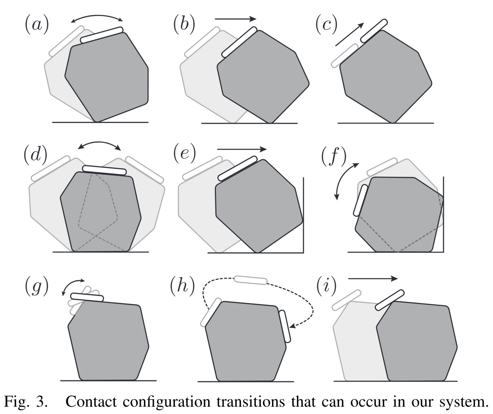
N. Doshi, O. Taylor, and A. Rodriguez, “Manipulation of unknown objects via contact configuration regulation,” in 2022 International Conference on Robotics and Automation (ICRA). IEEE, 2022, pp. 2693–2699.
Methods for planning over contact
Offline Contact-Implicit Planning
Idea: Include contact as a decision variable and handle nonconvexity by solving the problem offline.
- Add complementarity constraint violation to the objective for enforcement at the limit of convergence
- Solve the nonlinear program with methods such as SQP or interior point
Methods for planning over contact
Learning-Based Methods
Idea: Do not model contact, learn a model-free reinforcement learning policy to accomplish the task.
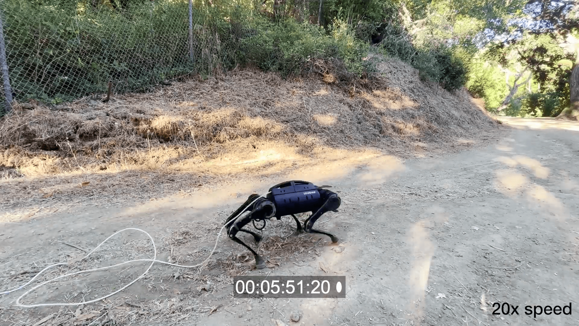
L. Smith, I. Kostrikov, and S. Levine, “A walk in the park: Learning to walk in 20 minutes with model-free reinforcement learning,” arXiv preprint arXiv:2208.07860, 2022.
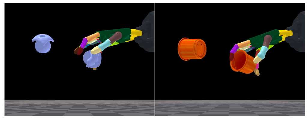
T. Chen, J. Xu, and P. Agrawal, “A system for general in-hand object re-orientation,” in Conference on Robot Learning. PMLR, 2022, pp. 297–307.
Methods for planning over contact
Contact-Implicit MPC
Idea: Include contact as a decision variable in an online MPC policy
- Can adapt to disturbances online
- Can synthesize or re-synthesize contact trajectories without prior-specification or another planning layer
Problem: Need to reformulate contact dynamics to solve optimal control online
Preliminaries and Notation
2
- Related work on contact
- Preliminaries
- Contact-implicit literature review
- Overview of methods analyzed
- Experiments and Discussion
- Future Work
2. Preliminaries
Optimal Control: Problem Formulation
Task: What we want the robot to achieve
Objective: An expression of how close we are to task success
State: Values that define where the robot is in space
Input: Torques and forces sent to the robot actuators
c(x,u)
x
u
Dynamics: How state changes over time, given inputs
f(x,u)

Optimal Control Problem Formulation
Concept: Find the optimal input (and state) trajectory that minimizes cost over time (achieves task success), subject to the dynamics of the system.
\begin{align*}
\min_{x_t, u_t} \quad & \sum_{t=0}^T c(x_t, u_t)\\
\textrm{s.t.} \quad & x_{t+1} = f(x_t, u_t) \\
\quad & x_0 = x_{\textrm{init}}, x_T = x_{\textrm{des}} \\
\quad & \textrm{(workspace and control limits)}
\end{align*}
optimal trajectory
system dynamics
cost over time
Discrete time problem:
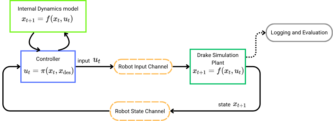
Model Predictive Control
Re-solve the optimal control problem at every timestep to use it as an online policy.
- Receive current state measurement
- Solve for optimal trajectory
- Execute first action in trajectory
- Allow dynamics to evolve for one timestep.
x_t
\{u_k\}_{t:(t+T)}
u_t
x_{t+1} = f(x_t, u_t)
\min_{x_t,u_t} \sum_{k=0}^T c(x_k, u_k)\\
\textrm{s.t.} \quad x_0 = x_t \\ \quad x_{t+1} = f^*(x_t,u_t)
x_{t+1}
x_t
\{u_k\}_{t:(t+T)}
u_t
x_{t+1}
controller
plant
Linearized Trajectory Optimization
Goal: Solve the optimal control problem using fast linear and convex solvers.
\begin{align*}
\min_{x_t, u_t} \quad & \sum_{t=0}^T x_t^\top Qx_t + u_t^\top R u_t\\
\textrm{s.t.} \quad & x_{t+1} = Ax_t + Bu_t \\
\quad & Ex_t + Hu_t = 0 \\
\end{align*}
f(x_t,u_t) \approx Ax_t + Bu_t
Use a quadratic cost term:
c(x_t,u_t) = x_t^\top Qx_t + u_t^\top R u_t\\
Q\succeq 0, \quad R\succeq 0
Linearize the system dynamics:
Linearize equality constraints:
Ex_t + Hu_t = 0
Robot Dynamics: The Manipulator Equation
The manipulator equation expresses force balance in a robotic system.
M(q)\ddot{q} + C(q,\dot{q}) = Bu + J(q)^\top \lambda
inertial force
Coriolis and gravity terms
contact forces
generalized torques
q_1
q_4
q_3
q_2
q = \begin{Bmatrix}q_1 \\ q_2 \\ q_3 \\ q_4 \end{Bmatrix}
generalized position vector
Contact Complementarity
distance to surface
sliding velocity
contact force
\lambda^{\textrm{n}}
\lambda^{\textrm{t}}
\varphi(q)
J^{\textrm{tan}}(q)\dot{q}
\lambda^{\textrm{n}}
\Vert\lambda^{\textrm{t}}\Vert \leq \mu \lambda^{\textrm{n}}
for 0 sliding velocity
\mu
Contact Complementarity
distance to surface
sliding velocity
contact force
\lambda^{\textrm{n}}
\lambda^{\textrm{t}}
\varphi(q)
J^{\textrm{tan}}(q)\dot{q}
\lambda^{\textrm{n}}
\Vert\lambda^{\textrm{t}}\Vert \leq \mu \lambda^{\textrm{n}}
\newcommand{\normforce}{\lambda^\textrm{n}}
\newcommand{\tanforce}{\lambda^\textrm{t}}
\varphi(q) \hspace{2pt} \perp \hspace{2pt} \normforce
\newcommand{\normforce}{\lambda^\textrm{n}}
\newcommand{\tanforce}{\lambda^\textrm{t}}
\textrm{contact velocity} \hspace{2pt} \perp \hspace{2pt} \mu\normforce - \Vert \tanforce\Vert
\geq 0
0\leq
\implies\quad 0\leq \lambda \perp \psi(q,\dot{q},u,\lambda)\geq 0
0\leq
\geq 0
Contact Dynamics and Impact
velocity
time
\Delta \dot{q} = M^{-1}J^\top \Lambda
\dot{q}
t
\lambda_0
contact force
time
t
At the limit of instantaneous impact (a rigid body system) the contact force over time can be represented with the Dirac delta function:

t_0
\lambda
\lambda(t) = \lambda_0\delta(t+t_0)
Formulate contact force in discrete time:
x_{t+1} = Ax_t + Bu_t + D\lambda_t + d \\
0\leq \lambda_t \perp Ex_t + F\lambda_t + Hu_t \geq 0\\
\ddot{q}(t) = f(q(t), \dot{q}(t), u(t), \lambda(t))\\
0\leq \lambda(t) \perp \varphi(q(t)) \geq 0\\
\lambda(t) = \sum_{i=0}^m\lambda_i\delta(t+t_i)
x = \begin{Bmatrix} q \\ \dot{q} \end{Bmatrix}
\dot{x} = \begin{Bmatrix} \dot{q} \\ \ddot{q} \end{Bmatrix}
Timestepping schemes avoid Dirac-deltas in dynamics constraints. Originally:
Linear Complementarity System (LCS)
Attempt: Mixed Integer Quadratic Program (MIQP)
Minimize the cost over all contact modes separately to search for the optimal sequence and trajectory
c_t = \begin{Bmatrix}c_0 \\ c_1 \\ \vdots \\ c_n \end{Bmatrix}_t \in \{0,1\}
Define binary contact decision variable for n contact pairs:
0\leq Ex_t + F\lambda_t + Hu_t \perp \lambda_t \geq 0
0\leq \lambda_t \leq (\mathbf{1} - c_t)M\\
0\leq Ex_t + F\lambda_t + Hu_t + c \leq c_tM
c_t \in \{0,1\}^n
nonconvex constraint:
convex constraints:
nonconvex constraint:
becomes
Attempt: Mixed Integer Quadratic Program (MIQP)
Problem: Worst case solve cost is exponential with time horizon and number of contacts
c_0
c_{0,1}
c_{0,1,1}
c_{0,1,0}
c_{0,0}
c_{0,0,1}
c_{0,0,0}
\textrm{...}
\textrm{...}
\textrm{...}
\textrm{...}
\textrm{...}
t_n
t_{n+1}
t_{n+2}
\textrm{...}
For one contact and binary contact modes:
1 (contact)
0 (free)
2^{Nn_\lambda}
worst case computation
Contact-Implicit MPC Problem
\begin{align*}
\min_{x_t, u_t, \lambda_t} \quad & \sum_{t=0}^T x_t^\top Qx_t + u_t^T R u_t\\
\textrm{s.t.} \quad & x_{t+1} = Ax_t + Bu_t + D\lambda_t + d \\
\quad & 0 \leq \lambda_t \perp Ex_t + F\lambda_t + Hu_t + c \geq 0 \\
\quad & x_0 = x_{\textrm{init}}, \textrm{ other workspace/control limits} \\
\end{align*}
Challenge: Complementarity constraint is nonconvex, so problem cannot be solved as-is with available convex and linear solvers.
We must modify the optimal control problem in some way to make this problem work with MPC.
Literature Review
3
- Related work on contact
- Preliminaries
- Contact-implicit literature review
- Overview of methods analyzed
- Experiments and Discussion
- Future Work
3. Contact-implicit literature review
Literature Review
There are many ways to reformulate contact dynamics for MPC. Many fall under three categories:
-
Sampling-based methods: Try a set of random inputs, allowing for sampling of other contact modes
-
Differentiable contact models: Add a small relaxation to the contact force Jacobian at contact boundaries, allowing for solutions to cross modes by indicating "force at a distance"
- Contact force -- dynamics disparity: Allow the controller to separately solve for desired contact and feasible dynamics, and then reconcile the conflict
Literature Review
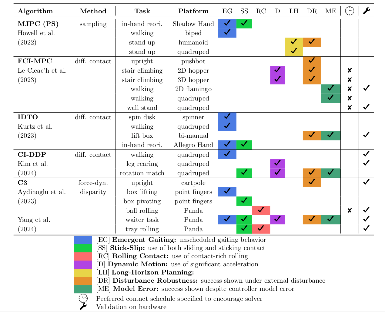
Different papers emphasize different qualities of their controller solutions. Some qualities that were commonly highlighted were:
- Emergent gaiting behavior
- Effective use of both sticking and sliding friction regimes
- Ability to use rolling contact and maintain contact force
- Use of significant acceleration (jumping, tossing, kicking)
- Long horizon solutions that aren't susceptible to local minima far from the goal
- Robustness to force disturbance and model error
- Ability to fully synthesize contact online with no reference trajectory
Literature Review
Literature Review
There is difference across authors about which solver qualities are important to achieve.
Goal: Evaluate multiple controllers on the exact same tasks to achieve a true comparison.
What makes a good benchmark?
Benchmark tasks should:
-
demonstrate important abilities that are needed for many tasks
- differentiate the strengths and weaknesses of different fundamental approaches.
Goal of this project: Provide an apples-to-apples comparison of different contact-implicit controllers on a set of tasks.
Methods Analyzed
4
- Related work on contact
- Preliminaries
- Contact-implicit literature review
- Overview of methods analyzed
- Experiments and Discussion
- Future Work
4. Overview of methods analyzed
Methods Evaluated
- Sampling-based method: MuJoCo MPC
T. Howell, N. Gileadi, S. Tunyasuvunakool, K. Zakka, T. Erez, and Y. Tassa, “Predictive sampling: Real-time behaviour synthesis with mujoco,” 2022
- Differentiable contact model: Fast Contact-Implicit MPC
S. Le Cleac’h, T. A. Howell, S. Yang, C.-Y. Lee, J. Zhang, A. Bishop, M. Schwager, and Z. Manchester, “Fast contact-implicit model predictive control,” IEEE Transactions on Robotics, vol. 40, pp. 1617–1629, 2024.
- Force-Dynamics disparity: C3
A. Aydinoglu, A. Wei, W.-C. Huang, and M. Posa, “Consensus complementarity control for multicontact mpc,” IEEE Transactions on Robotics, vol. 40, pp. 3879–3896, 2024.
Sampling: MuJoCo MPC (MJPC)
The MuJoCo simulator is able to resolve contact force realistically and stably in continuous time.
With access to fast realistic contact modeling, MuJoCo MPC uses the MuJoCo simulation to evaluate randomized inputs to choose the best one for the task.
This approach does not solve for the optimal control, but rather emphasizes solutions close enough to optimal sent at a faster control rate.
Algorithm:
- Sample N variations on a nominal input trajectory
- Simulate each input trajectory forward in parallel
- Evaluate the cost of each rollout
- Choose the best rollout to set as the new nominal policy
MuJoCo MPC (MJPC)
- Sample N variations on a nominal input trajectory
- Simulate each input trajectory forward in parallel
- Evaluate the cost of each rollout
- Choose the best rollout to set as the new nominal policy
u_0
u_1
u_{T-1}
u_T
cubic spline in input space
u_1'
u''_1
u''_T
u_T'
\pi_1 = \argmin_{\{u_t\}}\begin{cases}
c(\{x_t\}, \{u_t\})\\
\textcolor{green}{c(\{x'_t\}, \{u'_t\})}\\
\textcolor{blue}{c(\{x''_t\}, \{u''_t\})}
\end{cases}
\pi_0 = \{u_t\}_{0:T}
Differentiable Contact: Fast Contact-Implicit MPC (FCIMPC)
Rigid contact: No gradient for contact constraint
Soft contact: Gradient for contact constraint allows planner to make and break new contacts
\varphi
\lambda
\varphi
\lambda
Differentiable Contact: Fast Contact-Implicit MPC (FCIMPC)
Idea: Create a soft-contact LCP, solve trajectory quickly with pre-factorized solver components
- Use interior-point methods to simulate soft contact for planning, calculating contact gradients with implicit differentiation
- Solve the optimal control problem with direct collocation
To achieve success, many examples need a reference contact trajectory computed offline. For this evaluation, a reference is not provided.
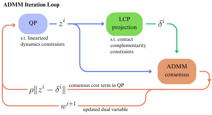
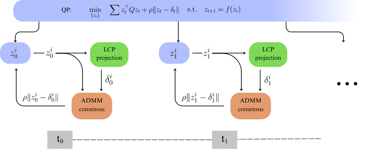
Force-Dynamics Disparity: Consensus Complementarity Control (C3)
-
QP Step: Minimize objective and consensus with projection, subject to dynamics between timesteps
- Projection Step: Minimize solution distance to step (1), subject to complementarity constraints
Idea: Allow contact force to conflict with feasible dynamics, and iteratively resolve this conflict with ADMM consensus
Consensus Complementarity Control (C3)
Alternate solving for best positions given desired contact force, and best desired contact force given objective and agreement with position
Consensus Complementarity Control (C3)
Key Differences
| Controller has contact model? | Controller uses rigid contact? | Only uses local contact pairs? | Solution minimizes objective analytically? | Decision variables | Solver hyperparameters | |
|---|---|---|---|---|---|---|
| MJPC |
|
sample variance | ||||
| FCIMPC |
|
complementarity relaxation | ||||
| C3 |
|
consensus parameters |
u_t
x_t, u_t, \lambda_t
x_t, u_t, \lambda_t
Experiments
5
- Related work on contact
- Preliminaries
- Contact-implicit literature review
- Overview of methods analyzed
- Experiments and Discussion
- Future Work
5. Experiments and Discussion
Setup
Tasks
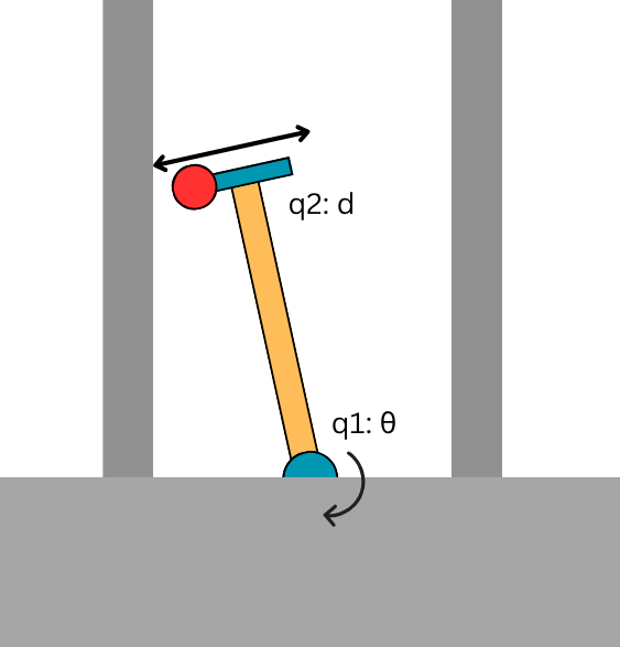
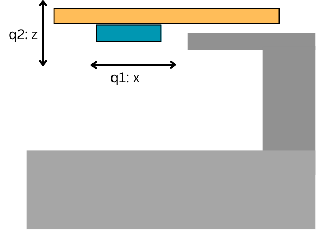
Pushbot
2D Waiter
Task Insights
Pushbot:
- Robustness to disturbance
- Ability to handle unstable equilibrium
- High acceleration / dynamic impact
2D Waiter:
- Use of sticking and sliding contact
- Capacity for emergent gaiting behavior
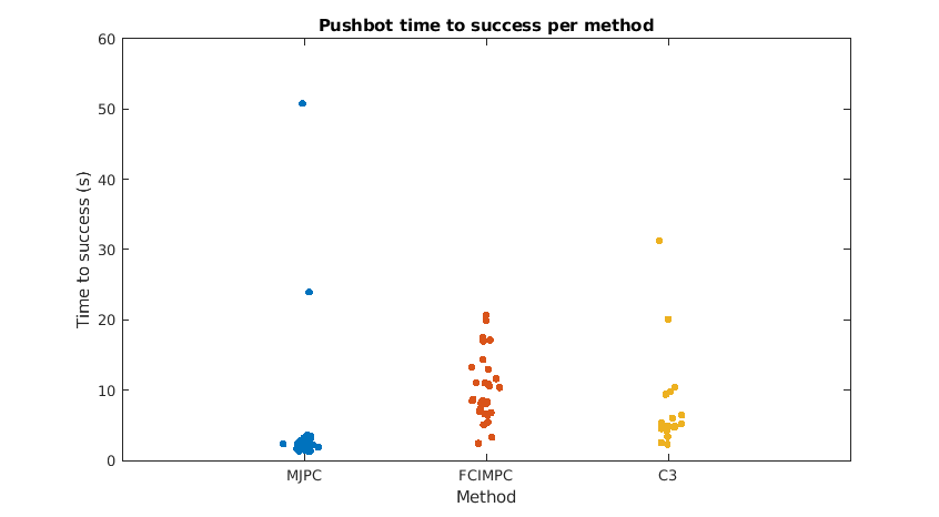
Solution Quality: Time to Success
- MuJoCo MPC was often fastest to a solution, but was susceptible to "bad luck" due to sampling numerics
- FCIMPC struggled to maintain equilibrium outside of its native simulation which exactly matches the controller dynamics
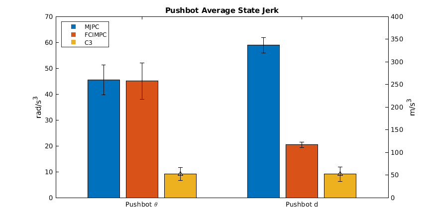
Solution Quality: Trajectory Jerk
- MuJoCo MPC showed highest jerk due to non-smooth nature of sample jitter in solution
- C3 showed the smallest jerk and relied on multiple, low force pushes on the wall to balance upright
Solution Quality: Average Contact Force
- FCIMPC used the most contact force overall, due to the soft-contact model used in the controller which leads to higher-impact contact on the robot than was solved for

Solution Quality Takeaways
- MJPC does not have true guarantees on performance even for simple problems.
- MJPC does well on a wide range of tasks, especially those that do not require small or precise motions, but could benefit from additional motion smoothing especially for real-world applications.
- FCIMPC performs well for tasks that just require small contact deviations from a nominal plan. Contact is often only made when surfaces are close enough to the robot, due to the soft contact model.
- FCIMPC can become stuck in local minima very easily
- C3 uses less force but makes contact more often than the other methods.
- C3 gets stuck in local minima less due to solving complementarity with an MIQP (being able to see all contact pairs)
Solver Sensitivity: Cost Weight Variance
MJPC was significantly more robust to variances in cost weight terms Q and R than C3 (and FCIMPC). Unlike the other two methods, MJPC does not use the cost terms analytically to find a solution.
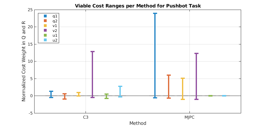
c = x^\top Q x + u^\top R u \implies \nabla_xc = 2Qx, \quad \nabla_uc = 2Ru
For trajectory optimization methods like C3 and FCIMPC, Q and R appear in the cost gradient and therefore affects the numerical conditioning of the solver:
Current Challenges
The waiter task currently faces some challenges to reasonable task success.
- FCIMPC only converges on a solution under a narrow range of cost weights and solver parameters. Tuning within this range to achieve task success is difficult.
- From the original paper: "Generating high-quality reference trajectories is crucial for CI-MPC... Ultimately, for CI-MPC to be of practical value, generation of references trajectories, even in the offline setting, must be improved."
- From the original paper: "Generating high-quality reference trajectories is crucial for CI-MPC... Ultimately, for CI-MPC to be of practical value, generation of references trajectories, even in the offline setting, must be improved."
- C3 requires close tracking and balance of the separate trajectories for state and expected contact force, as these trajectories may conflict with each other.
- Prior work also used an intermediary operational space controller (OSC) to help reconcile conflicts into a robot input trajectory. This work currently uses a PD controller which may require more extensive adjustment for success.
- Prior work also used an intermediary operational space controller (OSC) to help reconcile conflicts into a robot input trajectory. This work currently uses a PD controller which may require more extensive adjustment for success.
- The solution performance for MJPC drops considerably when deployed in a different simulator, which has been observed across multiple tasks. Closer tracking of solution trajectories may be necessary for success on this problem, which requires correct handling of friction.
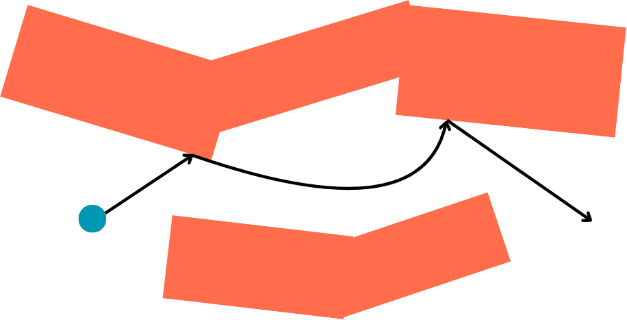
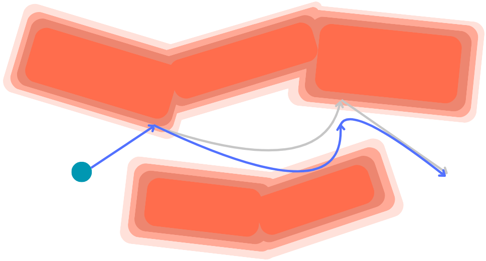
Ongoing and Future Work
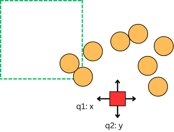
Things that are being explored via the waiter task and a third circle corralling task:
- Local linearized controller performance in non-convex free space (i.e. in the negative space of circles) both with and without a preferred contact schedule.
-
Controller performance as number of inputs / states scales, specifically how each controller's computation cost grows and the performance of sampling-based planning
-
Role of a lower level controller for C3 and MJPC, specifically, ablations and sensitivity analysis
- Use of sticking and sliding contact, specifically the difference between planned sticking and sliding compared to executed
Appendix
I.
Optimal Control Problem Formulation
Concept: Find the optimal input (and state) trajectory that minimizes cost over time (achieves task success), subject to the dynamics of the system.
\begin{align*}
\min_{x_t, u_t} \quad & \int_0^T c(x_t, u_t)dt\\
\textrm{s.t.} \quad & \dot{x} = f(x_t, u_t) \\
\quad & x_0 = x_{\textrm{init}}, x_T = x_{\textrm{des}} \\
\quad & \textrm{(workspace and control limits)}
\end{align*}
optimal trajectory
system dynamics
cost over time
Continuous time problem:
Contact Dynamics and Impact
For soft contact events, contact force imparts an impulse across the time of contact:
velocity
time
\Delta \dot{q} = M^{-1}J^\top \int_0^T \lambda_0 dt
\dot{q}
t

T
contact period
time
t
contact force
\lambda
\lambda_0
quals-presentation-draft1
By Grey Sarmiento


