COMP2521
Data Structures & Algorithms
Week 3.2
Balancing Binary Search Trees
Author: Hayden Smith 2021
In this lecture
Why?
- Binary Search Trees will often slowly lead to more imbalanced trees, so we need to develop strategies to prevent that.
What?
- Tree Rotations
- Insertions at root
- Tree partitioning
BST balance as it grows
When you insert into a BST, there are two extreme cases:
- Best case: Keys inserted in pre-order such that it is perfectly balanced
- Tree height = log(n)
- Search cost = O(log(n))
- Worst case: Keys inserted in ascending or descending order such that it is completely unbalanced:
- Tree height = O(n)
- Search cost = O(n)
In reality, the average case is a mix between these too. This is still a search cost of O(log(n)), though the real cost is more than the best case
Balanced BST
The formal definition for a weight-balanced BST is a tree that, for all nodes:
- ∀ nodes, abs(#nodes(LeftSubtree) - #nodes(RightSubtree)) < 2
The formal definition for a height-balanced BST is a tree that, for all nodes:
- ∀ nodes, abs(height(LeftSubtree) - height(RightSubtree)) < 2
Operations for more balanced BSTs
There are 4 key operations we will look at that help us balance
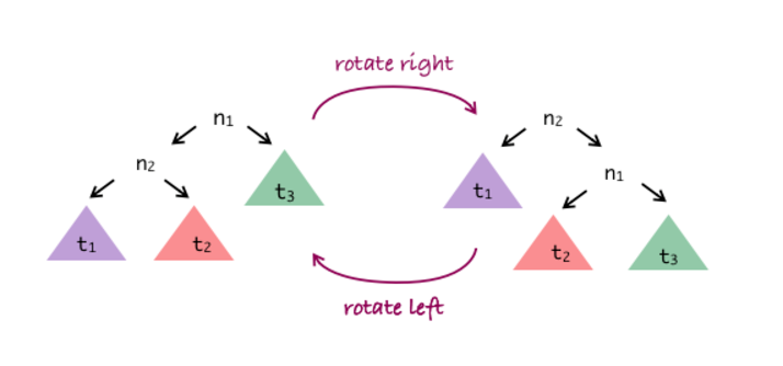
Left rotation
Move right child to node, then rearrange links to retain order
Right rotation
Move left child to node, then rearrange links to retain order
Insertion at root
Each new item added at root node. (Added at leaf then rotated up)
Partition
Rearrange tree around specified node (push to root)
Tree rotation (practical)
5
3
4
2
6
5
3
4
2
6
Rotate (5) right
5
3
4
2
6
1
2
3
Tree rotation (practical)
5
3
4
2
6
5
3
4
2
6
Rotate (3) left
1
2
3
5
3
4
2
6
Tree rotation (practical)
Rotate (5) right
Rotate (3) left
5
3
4
6
5
3
4
2
6
2
Tree rotation (theoretical)
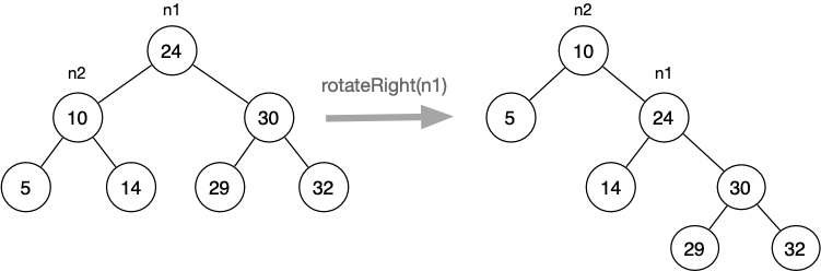
Formally the process for rotating is (for right rotation):
- n1 is current root; n2 is root of n1's left subtree
- n1 gets a new left subtree, which is n2's right subtree
- n1 becomes root of n2's new right subtree
- n2 becomes new root
- n2's left subtree is unchanged
- Left rotation is just swapping left/right above
Tree rotation (example)
Tree rotation algorithms
rotateRight(root):
    newRoot = (root's left child)
    if (root) is empty or (newRoot) is empty:
        return root
    (Root's left child) should now point to (newRoot's right child)
    (newRoot's right child) should now point to root
    return newRoot
rotateLeft(root):
newRoot = (root's right child)
if (root) is empty or (newRoot) is empty:
return root
(Root's right child) should now point to (newRoot's left child)
(newRoot's left child) should now point to root
return newRootTree rotation algorithms
- When looking at a single rotation:
- Cheap cost O(1)
- Rotation requires simple, localised pointer arrangement
- Sometimes rotation is applied from leaf to root, along one branch
- Cost of this is O(height)
- Payoff is improved balance which reduces height
- Pushes search cost towards O(log n)
Insertion at root
Approach: Insert new items at the root
- Method: Insert new node as leaf normally in tree, then lift new node to top by rotation
- Benefit(s): Recently-inserted items are close to the root, therefore lower cost if recent items are more likely to be searched.
- Disadvantages: Requires large-scale re-arrangement of tree
Insertion of 24 at root
10
5
14
30
32
29
24
10
5
14
30
32
29
24 as a leaf
Insertion of 24 at root
10
5
14
30
32
29
24
Rotate 29 right
10
5
14
30
32
29
24
Insertion of 24 at root
10
5
14
30
32
29
24
Rotate 30 right
10
5
14
30
32
29
24
Insertion of 24 at root
10
5
14
30
32
29
24
Rotate 14 left
10
5
14
30
32
29
24
Insertion of 24 at root
10
5
14
30
32
29
24
Rotate 10 left
10
5
14
30
32
29
24
Insertion at root
Pseudocode
insertAtRoot(tree, item):
    root = get root of "tree"
    if tree is empty:
        tree = new node containing item
    else if item < root's value:
        (tree's left child) = insertAtRoot((tree's left child), item)
        tree = rotateRight(tree)
    else if item > root's value:
        (tree's right child) = insertAtRoot((tree's right child), item)
        tree = rotateLeft(tree)
    return tree
Insertion at root
- Complexity: O(h)
- Cost is doubled in reality though, as you have to traverse down then traverse up
- Insertion at root has a higher tendency to be balanced, but no balance is guaranteed.
-
For applications where the same element is looked up many times, you can only consider moving a node to the root when it's found during a search.
- This makes lookup for recently accessed items very fast
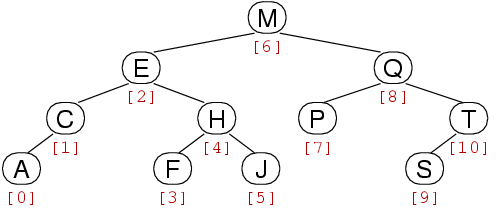
Tree Partitioning
partition(tree, index)
Rearranges tree so that element with index i becomes root. Indexes are based on in-order.
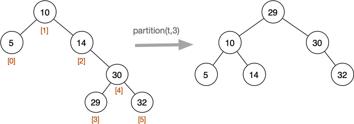
Tree Partitioning Example
If we partition the middle index, quite often we'll get something more balanced.
Tree Partitioning
Pseudocode
Pseudocode
partition(tree, index)
    m = # nodes in the tree's left subtree
    if index < m:
        (tree's left subtree) = partition(tree's left subtree, index)
        tree = rotateRight(tree)
    else if index > m:
        (tree's right subtree) = partition(tree's right subtree, index - m - 1)
        tree = rotateLeft(tree)
    return tree
Tree Partitioning Complexity
Time complexity similar to insert-at-root. Gets faster the more we partition closer to the root.
Periodic Rebalancing
A simple approach to using partition selectively.
Let's rebalance the tree every k inserts
periodicRebalance(tree, index)
    tree = insertAtLeaf(tree, item)
    if #nodes in tree % k == 0:
        tree = partition(tree, middle index)
    return tree
Periodic Rebalancing
The problem? To find the #nodes in a tree we need to do a O(n) traversal which can be expensive to do often.
Is is going to be "better" to store the nodes in any given subtree within the node itself? Yes? No?
typedef struct Node {
   int  data;
   int  nnodes;      // #nodes in my tree
   Tree left, right; // subtrees
} Node;
Feedback

COMP2521 21T2 - 3.2 - Balancing BSTs
By haydensmith


