Constrained Dynamics in Conformal and Projective Geometric Algebra

Hugo Hadfield, Joan Lasenby

University Of Cambridge,

Signal Processing and Communications Laboratory

Speaker: Hugo Hadfield
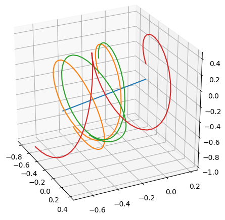
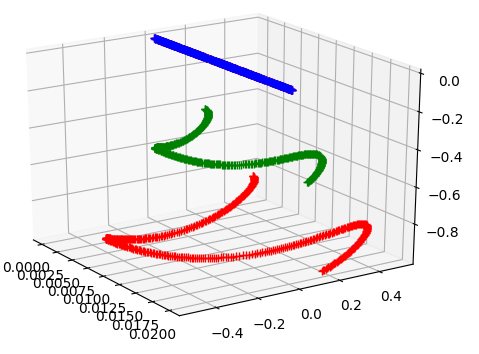
Forces and Moments

  • The Screw Theory perspective views forces as lines:
  • To have the equivalent in PGA you can simply swap \(n_\infty\) for \(e_0 \)
  • Adding lines together gives screws
  • Antiparallel force lines add to give a force couple, a pure moment (or torque or whatever you want to call it!)
  • Form of a moment:
  • Form of a screw:
\newcommand{\ninf}{n_{\infty}} F = \lambda[\hat{m}I_3 - (p\wedge\hat{m})I_3\ninf]

force magnitude

force direction

3d point through which the line passes

B = be_0
B = bn_\infty
\newcommand{\ninf}{n_{\infty}} S = mI_3 - ( p \wedge m)I_3\ninf + h\hat{m}\ninf
\newcommand{\ninf}{n_{\infty}} S = mI_3 - ( p \wedge m)I_3e_0 + h\hat{m}e_0

Static Equilibrium

  • Static Equilibrium for a rigid body occurs when all the forces and moments about the centre of mass sum to 0:
\sum_i F_i + \sum_j M_j = 0
\sum_k S_k = 0
  • We could also think of all the force and moments as special cases of screws and so:

Momentum, Inertia and Velocity (CGA)

  • The unbalanced resultant wrench acting on a rigid body is defined as the derivative of the screw momentum \(\Omega\)
  • The mapping between screw momentum and screw velocity is produced by the inertia tensor
\Omega = M(\dot{B}) = m\sum_{i=1}^{i=3} \left[ (\dot{B}\cdot t^i)l_i + \gamma_i(\dot{B}\cdot l^i)t_i \right]
M^{-1}(\Omega) = \dot{B} = \frac{1}{m}\sum_{i=1}^{i=3}\left[ \frac{1}{\gamma_i}(\Omega\cdot t^i)l_i + (\Omega\cdot l^i)t_i \right]
l_i = e_iI_3, \,\,\,\, l^i = -e_iI_3 \\ t_i = e_i\wedge n_\infty, \,\,\,\, t^i = e_i\wedge n_0
W_r = \sum W_i = \frac{\partial\Omega}{\partial t}

Momentum, Inertia and Velocity (PGA)

  • In PGA we need to use an alternative to reciprocal frames to describe the principal screws and so use a pseudo-reciprocal frame a la Gunn []
l_i = e_iI_3, \,\,\,\, l^i = e_i\wedge e_0 \\ t_i = e_i\wedge e_0, \,\,\,\, t^i = e_iI_3
\newcommand{\la}{\langle} \newcommand{\ra}{\rangle} \newcommand{\nn}{\nonumber} \newcommand{\ninf}{n_{\infty}} \newcommand{\einf}{e_{\infty}} \newcommand{\no}{n_{0}} \newcommand{\eo}{e_{0}} \newcommand{\wdg}{\wedge} \newcommand{\pdiff}[2]{\frac{\partial #1}{\partial #2} } \Omega = M(\dot{B}) = -m\sum_{i=1}^{i=3} \left[ \la \dot{B}\wedge l^i\ra_{e1230}l^i + \gamma_i\la \dot{B}\wedge t^i\ra_{e1230}t^i\right] \\ M^{-1}(\Omega) = \dot{B} = -\frac{1}{m}\sum_{i=1}^{i=3}\left[ \frac{1}{\gamma_i}\la \Omega\wedge l^i\ra_{e1230}l^i + \la \Omega\wedge t^i\ra_{e1230}t^i \right]
  • Or, defining a mapping \(J\), we can use a componentwise scaling A:
X^J = J(X) = J\left(\sum_i b_ix_i\right) = \sum_i J(b_ix_i)\\ \Omega = M(\dot{B}) = A[J(\dot{B})]

Free Dynamics

Y_t = \begin{bmatrix} R_t\\ \Omega_t \end{bmatrix}, \hspace{1em} \dot{Y_t} = \begin{bmatrix} \dot{R_t}\\ \dot{\Omega}_t \end{bmatrix} = \begin{bmatrix} -\frac{1}{2}R_t\dot{B}_t\\ R_tW_{bt}\tilde{R}_t \end{bmatrix}
  • We will set up our state at a given time as follows:
\dot{B} = M^{-1}[\tilde{R}\Omega R]
\dot{Y} = \begin{bmatrix} \dot{R}\\ \dot{\Omega} \end{bmatrix} = \begin{bmatrix} -\frac{1}{2}RM^{-1}[\tilde{R}\Omega R]\\ RW_{b}\tilde{R} \end{bmatrix}
  • Substitute in for the angular velocity:
  • And you can now plug this into your favourite initial value problem solver (eg. RK4) and simulate away!

The Free Spinning Cuboid

  • A cuboid set in motion spinning about its intermediate axis will not be stable in its rotation
  • Cuboid flips every so often, centre of mass (if moving) translates linearly as expected

Reaction Forces by Virtual Power

  • A common technique in constrained dynamics is that of virtual power
  • An virtual force \(T\) is imagined to align with the degree of freedom being constrained along with the condition that this force must be do no work in a given instant, ie. no virtual power
P = \dot{B}\wedge(\tilde{R}TR) = 0
\dot{P} = \ddot{B}\wedge(\tilde{R}TR) + \dot{B}\wedge\left(\dot{\tilde{R}}TR + \tilde{R}(\dot{T}R + T\dot{R})\right)
M^{-1}[W_b]\wedge(\tilde{R}TR) = - M^{-1}[\dot{\tilde{R}}\Omega R + \tilde{R}\Omega\dot{R}]\wedge(\tilde{R}TR) - \dot{B}\wedge\left(\dot{\tilde{R}}TR + \tilde{R}(\dot{T}R + T\dot{R})\right)

Multivector Pinning

  • Consider a point V in the world frame, and the same point but in the body frame, denoted U:
V = RU\tilde{R}, \,\,\,\,\,\,\, U = \tilde{R}VR
\dot{U} = \dot{\tilde{R}}VR + \tilde{R}(\dot{V}R + V\dot{R}) \\ \ddot{U} = \ddot{\tilde{R}}VR + 2\dot{\tilde{R}}(\dot{V}R + V\dot{R}) + \tilde{R}\ddot{V}R + 2\tilde{R}\dot{V}\dot{R} + \tilde{R}V\ddot{R}
  • Now we will allow the frame to move:
  • What if the frame can still move but we impose the restriction that \(\dot{U}\) and \(\dot{V}\) = 0?
0 =\ddot{\tilde{R}}VR + \tilde{R}V\ddot{R} + 2\dot{\tilde{R}}V\dot{R}
  • Can we take this equation and directly solve it to get the reaction forces at the point?

Multivector Pinning Leads to a Linear Problem

-\frac{1}{2}\ddot{B}U + \frac{1}{2}U\ddot{B} = \frac{1}{4}\dot{B}^2U + \frac{1}{4}U\dot{B}^2 - \frac{1}{2}\dot{B}U\dot{B}
  • Take our rotor equation and substitute in rotor time derivatives, leads to:
\ddot{B} = M^{-1}[\dot{\tilde{R}}\Omega R + \tilde{R}\Omega\dot{R}] + M^{-1}[W_b]
  • Differentiating our state derivative equation again leads to:
(U\times M^{-1}[W_b]) = \text{function of } R, \Omega, U
  • Substitute in and rearranging leads to a linear function of \(W_b\) which can be split as \(W_b = F + S\):
(U\times M^{-1}[F]) = -(U\times M^{-1}[S]) + \text{function of }R, \Omega, U

Reaction Wrench Force Basis

  • We want to solve for F:
  • F is a linear combination of the screw basis bivectors but it is not a full rank problem we need to provide a valid basis for the reaction wrench and can then solve via standard matrix methods
  • A valid basis for a point pin reaction force is three non-colinear forces force lines passing through the point
  • The pinning technique we have shown here will work for any multivector - but the user must provide a valid basis to solve it
(U\times M^{-1}[F]) = -(U\times M^{-1}[S]) + \text{function of }R, \Omega, U

Pinning in PGA

  • In PGA all of the flat elements are available to be pinned
    • Points (3 rotational dof)
    • Line (1 translational dof, 1 rotational dof)
    • Plane (2 translational dof, 1 rotational dof)
    • Direction vector  (3 translational dof)

Pinning in CGA

  • In CGA we have all of the flat blades of PGA available for pinning
    • Points (3 rotational dof)
    • Line (1 translational dof, 1 rotational dof)
    • Plane (2 translational dof, 1 rotational dof)
    • Direction vector  (3 translational dof)
  • But also we can also pin with the round blades
    • Point-pair (1 rotational dof)
    • Circle (1 rotational dof)
    • Sphere (3 rotational dof)

Pinning the Spinning Top

  • Pin the tip of a spinning top in body space to the origin in world space
  • Add gravity and give it a spin about its axis, exhibits precession and nutation as expected

Pinning the Physical Pendulum

  • We can verify we our physics with simple checks, one of the simplest being the small angle swinging time period of a uniform rod

Closed form predicted time period

Dynamic Pinning

  • It is also possible to pin parametric functions of multivectors in one frame to other parametric functions in another
  • This allows you to pin one moving object in one frame to a moving (or still of course) one in another
  • Simply relax constraint that \(\dot{U}\) and \(\dot{V}\) must be 0, and rearrange as before
  • Can solve with the same force basis as the static case
(U\times M^{-1}[F]) = \text{Some function of }R, \Omega, U, \dot{U}, \ddot{U}, V, \dot{V}, \ddot{V}, S

Dynamic Pinning

  • Here we start the pendulum still but drive the attachment point sinusoidally:

Pinning Linear Functions

  • It is also possible to pin linear functions between spaces. This time U is a linear function of the image of V in the body space:
U = A\left[\tilde{R}VR\right], \,\,\,\,\,\,\,\, \dot{U} = A\left[\dot{\tilde{R}}VR + \tilde{R}(\dot{V}R + V\dot{R})\right]\\ \ddot{U} = A\left[ \ddot{\tilde{R}}VR + 2\dot{\tilde{R}}(\dot{V}R + V\dot{R}) + \tilde{R}\ddot{V}R + 2\tilde{R}\dot{V}\dot{R} + \tilde{R}V\ddot{R} \right]
  • Substitute and rearrange as before:
A\left[(\tilde{R}VR)\times M^{-1}[F]\right] = A\left[-((\tilde{R}VR)\times M^{-1}[S]) + \text{function of }R, \Omega, U, \dot{U}, \ddot{U}, V, \dot{V}, \ddot{V} \right]
  • Again this is linearly solvable but requires a little thought as to what basis is required to solve the problem

Pinning Linear Functions

  • For example: V might be a circle, \(\dot{U}\) and \(\dot{U}\) might be 0, and A an outer product with a body frame point P:
A[X] \mapsto P\wedge X
  • Forces world frame circle always incident with the body frame point, but otherwise allows free movement!
  • For the circle-point incidence case this produces a 4dof system

Pinning Linear Functions

  • Pinning the outer product of a CGA sphere and point to the value 0 gives a 5dof system 

Why is Pinning Multivectors Useful?

  • No need to differentiate virtual power constraints for curved objects


  • Setting up the problem is very geometric and intuitive


  • Should generalise to higher dimensional algebras very easily, anything with motors and geometric primitives is a good target

Future Work

  • Higher dimensional algebras with more richness provide non trivial pinning primitives, eg. Can we pin dynamic rigid bodies to DCGA quadrics directly?
  • Currently we integrate the rotor R, over time with simple integration methods this will wander off the rotor manifold. Can we re-phrase entirely in the bivector (lie algebra) domain?
  • Game engines often use impulse driven physics engines, can we bring them into this framework?
  • There is a lot of very good and well established work in Screw Theory applied to articulated rigid body dynamics, swept surfaces, etc. Let's bring more into GA to make it understandable (good places to start: Helmut Pottmann, Roy Featherstone)

Conclusions

  • Screw Theory based dynamics embeds into both CGA and PGA very easily
  • Virtual power constraints work as expected in the GA formulation
  • Multivector pinning offers an alternative viewpoint on constraints and allows the geometric richness of an algebra to shine
  • Dynamic linear multivector function pinning is a very flexible way of defining constraints on a rigid body system

Constrained Dynamics in Conformal and Projective Geometric Algebra

By Hugo Hadfield

Constrained Dynamics in Conformal and Projective Geometric Algebra

  • 951