Geometric Algebra and Self Driving Cars

Hugo Hadfield, 2021

What is a Self Driving Car?

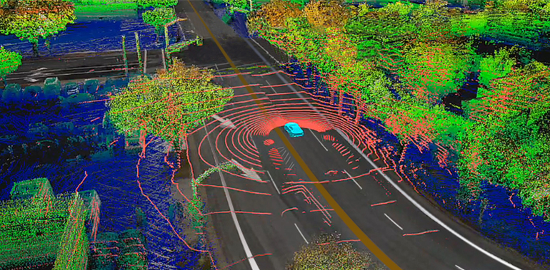
Several high definition cameras

Automotive RADAR

Speed and steering sensors
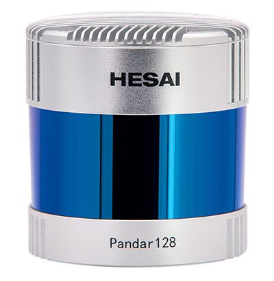
LIDAR system

GPS and IMU/INS

Bundle Adjustment

  • Where are the cameras relative to each other?


  • What does the scene look like in 3D?


  • One of the most important problems in applied computer vision

Bundle Adjustment

R_i = \exp{\Phi_i}\\ Y_j = up(y_j)\\ L_{ij} = n_o\wedge (R_iY_j\tilde{R_i})\wedge n_\infty \\ P_{ij} = L_{ij}\vee \Pi \\ P_{ij}\wedge n_\infty = \lambda(p_{ij}\wedge n_\infty - e_{45}) \\ C = \sum_{i}\sum_{j} \left( p_{ij} - \hat{p}_{ij} \right)

Minimise \(C\) with respect to \(\Phi_i\) and \(Y_j\)

Bundle Adjustment

Minimise \(C\) with respect to \(\Phi_i\) and \(Y_j\)

This is a Convex Optimisation Problem


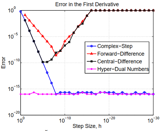
For derivatives we can simply construct the clifford algebra over the complex numbers or over the dual numbers!

R_i = \exp{\Phi_i}\\ Y_j = up(y_j)\\ L_{ij} = n_o\wedge (R_iY_j\tilde{R_i})\wedge n_\infty \\ P_{ij} = L_{ij}\vee \Pi \\ P_{ij}\wedge n_\infty = \lambda(p_{ij}\wedge n_\infty - e_{45}) \\ C = \sum_{i}\sum_{j} \left( p_{ij} - \hat{p}_{ij} \right)

Complex/Dual number  Autodiff

We can calculate automatic derivatives through complex/dual number autodiff


See the work of Jeffrey Fike:

http://adl.stanford.edu/hyperdual/

y = F(x) \quad h = 10^{-8} \\ F(x + hj) \approx y + hj\frac{dy}{dx}

Hyper Complex/Dual number GA isomorphisms

\mathbb{C}^n
Cl(n, n)
  • The hyper complex and hyper dual numbers have known isomorphisms to subalgebras of certain Clifford algebras


  • So long as you have a software package that can handle type stability for Clifford algebras over (a subset of communtative) Clifford algebras you get autodiff built in!

SLAM

If we take our collection of cameras on a drive they can repeatedly do bundle adjustments and build up a 3D map of the world!


We could even use multiple frames from a single camera moving through space

LIDAR DATA

LIDAR SLAM

  • At each point in time we get a point cloud
  • Align each point cloud with the previous one
  • Build up 3D map of the world and of how you have moved relative to it


  • But how do you align the (often quite sparse) point clouds?
  • Not many GA methods yet, interesting area of work!

Localisation to HD Maps

  • Most self-driving cars operate by localising themselves relative to high definition point cloud maps

Model Based Motion Filtering

Given a noisey sequence of measurements of the positions of a moving car how do you estimate its position at any point in time?

R_t = \exp{\Phi_t}

Describe each position with a rotor

Convex optimisation, minimising difference between position and measurment and function of the path

F(R_0, ... R_T) + \sum_t^T C(R_t, \hat{R_t})

Model Based Motion Filtering

\dot{\Phi} = -\frac{1}{4}(1 - \Phi)\Omega(1 + \Phi)

Describe the state of the car at a point in time with a vector

We include, combined position and rotation: \(\Phi\)

Combined linear and angular velocity: \(\Psi\)

Design a function that takes a given state and advances it one time step. Use this motion model to propogate uncertainty about the state of the car:

This is the basic setup required for an (extended/unscented) Kalman Filter

Model Based Motion Filtering

Set up a state like this:

\dot{\Phi}_k = \frac{1}{4}(1 - \Phi_k)\Omega_k(1 + \Phi_k) \\ \Phi_{k + 1} = \Phi_k + \dot{\Phi}_k\Delta T
\begin{bmatrix} \Phi \\ \Omega \end{bmatrix}
R_k = (1 - \Phi_k)(1 + \Phi_k)^{-1} \\ Y_j = up(y_j)\\ L_{kj} = n_o\wedge (R_kY_j\tilde{R_k})\wedge n_\infty \\ P_{kj} = L_{kj}\vee \Pi \\ P_{kj}\wedge n_\infty = \lambda(p_{kj}\wedge n_\infty - e_{45})

Set up a process function (Cayley kinematic equation):

Set up a measurement function:

Processing depth images

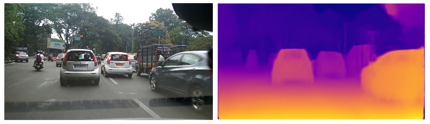
Given a depth image of the road, reject outliers and fit a plane

Monodepth machine learning models generate depth maps

  • Semantic segmentation to get the depth of the road area
  • Fit plane by looking for the eigen-blade of:
\sum_i P_i\Pi P_i

Simulation

  • Almost all self-driving companies use simulation for training and verification


  • Simulation systems tend to be similar to or to directly use games engines for physics and lighting


  • GA has a long history of being used in games and graphics!

Forces and Moments

  • The Screw Theory perspective views forces as lines:
  • To have the equivalent in PGA you can simply swap \(n_\infty\) for \(e_0 \)
  • Adding lines together gives screws
  • Antiparallel force lines add to give a force couple, a pure moment (or torque or whatever you want to call it!)
  • Form of a moment:
  • Form of a screw:
\newcommand{\ninf}{n_{\infty}} F = \lambda[\hat{m}I_3 - (p\wedge\hat{m})I_3\ninf]

force magnitude

force direction

3d point through which the line passes

B = be_0
B = bn_\infty
\newcommand{\ninf}{n_{\infty}} S = mI_3 - ( p \wedge m)I_3\ninf + h\hat{m}\ninf
\newcommand{\ninf}{n_{\infty}} S = mI_3 - ( p \wedge m)I_3e_0 + h\hat{m}e_0

Momentum, Inertia and Velocity (CGA)

  • The unbalanced resultant wrench acting on a rigid body is defined as the derivative of the screw momentum \(\Omega\)
  • The mapping between screw momentum and screw velocity is produced by the inertia tensor
\Omega = M(\dot{B}) = m\sum_{i=1}^{i=3} \left[ (\dot{B}\cdot t^i)l_i + \gamma_i(\dot{B}\cdot l^i)t_i \right]
M^{-1}(\Omega) = \dot{B} = \frac{1}{m}\sum_{i=1}^{i=3}\left[ \frac{1}{\gamma_i}(\Omega\cdot t^i)l_i + (\Omega\cdot l^i)t_i \right]
l_i = e_iI_3, \,\,\,\, l^i = -e_iI_3 \\ t_i = e_i\wedge n_\infty, \,\,\,\, t^i = e_i\wedge n_0
W_r = \sum W_i = \frac{\partial\Omega}{\partial t}

Momentum, Inertia and Velocity (PGA)

  • In PGA we need to use an alternative to reciprocal frames to describe the principal screws and so use a pseudo-reciprocal frame a la Gunn []
l_i = e_iI_3, \,\,\,\, l^i = e_i\wedge e_0 \\ t_i = e_i\wedge e_0, \,\,\,\, t^i = e_iI_3
\newcommand{\la}{\langle} \newcommand{\ra}{\rangle} \newcommand{\nn}{\nonumber} \newcommand{\ninf}{n_{\infty}} \newcommand{\einf}{e_{\infty}} \newcommand{\no}{n_{0}} \newcommand{\eo}{e_{0}} \newcommand{\wdg}{\wedge} \newcommand{\pdiff}[2]{\frac{\partial #1}{\partial #2} } \Omega = M(\dot{B}) = -m\sum_{i=1}^{i=3} \left[ \la \dot{B}\wedge l^i\ra_{e1230}l^i + \gamma_i\la \dot{B}\wedge t^i\ra_{e1230}t^i\right] \\ M^{-1}(\Omega) = \dot{B} = -\frac{1}{m}\sum_{i=1}^{i=3}\left[ \frac{1}{\gamma_i}\la \Omega\wedge l^i\ra_{e1230}l^i + \la \Omega\wedge t^i\ra_{e1230}t^i \right]
  • Or, defining a mapping \(J\), we can use a componentwise scaling A:
X^J = J(X) = J\left(\sum_i b_ix_i\right) = \sum_i J(b_ix_i)\\ \Omega = M(\dot{B}) = A[J(\dot{B})]

Free Dynamics

Y_t = \begin{bmatrix} R_t\\ \Omega_t \end{bmatrix}, \hspace{1em} \dot{Y_t} = \begin{bmatrix} \dot{R_t}\\ \dot{\Omega}_t \end{bmatrix} = \begin{bmatrix} -\frac{1}{2}R_t\dot{B}_t\\ R_tW_{bt}\tilde{R}_t \end{bmatrix}
  • We will set up our state at a given time as follows:
\dot{B} = M^{-1}[\tilde{R}\Omega R]
\dot{Y} = \begin{bmatrix} \dot{R}\\ \dot{\Omega} \end{bmatrix} = \begin{bmatrix} -\frac{1}{2}RM^{-1}[\tilde{R}\Omega R]\\ RW_{b}\tilde{R} \end{bmatrix}
  • Substitute in for the angular velocity:
  • And you can now plug this into your favourite initial value problem solver (eg. RK4) and simulate away!

Computer Graphics

GA Neural Networks

  • Are GA neural networks worthwhile? Quite a lot of hype in this area, would be good to see results!


  • What should GA neural networks look like mathematically
    • Activation functions are difficult to define


  • As far as I am aware no one has properly benchmarked GA NN against existing state of the art methods

Summary

  • We can build almost the entire self-driving stack in Geometric Algebra


  • Building self driving cars with GA is worthwhile because it is interdisciplinary and GA is a unifying framework


  • Still work to do in point cloud processing with GA


  • Still work to do in benchmarking GA neural network methods. Are they worthwhile at all?

Applications of Geometric Algebra in Self Driving Cars

By Hugo Hadfield

Applications of Geometric Algebra in Self Driving Cars

  • 54