


He Wang PRO
Knowledge increases by sharing but not by saving.
He Wang (王赫)
[hewang@mail.bnu.edu.cn]
Department of Physics, Beijing Normal University
On behalf of the KAGRA collaboration
In collaboration with Prof. Zhou-Jian Cao
Jan 10th, 2020
Key Laboratory of Computational Geodynamics, CAS
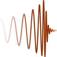
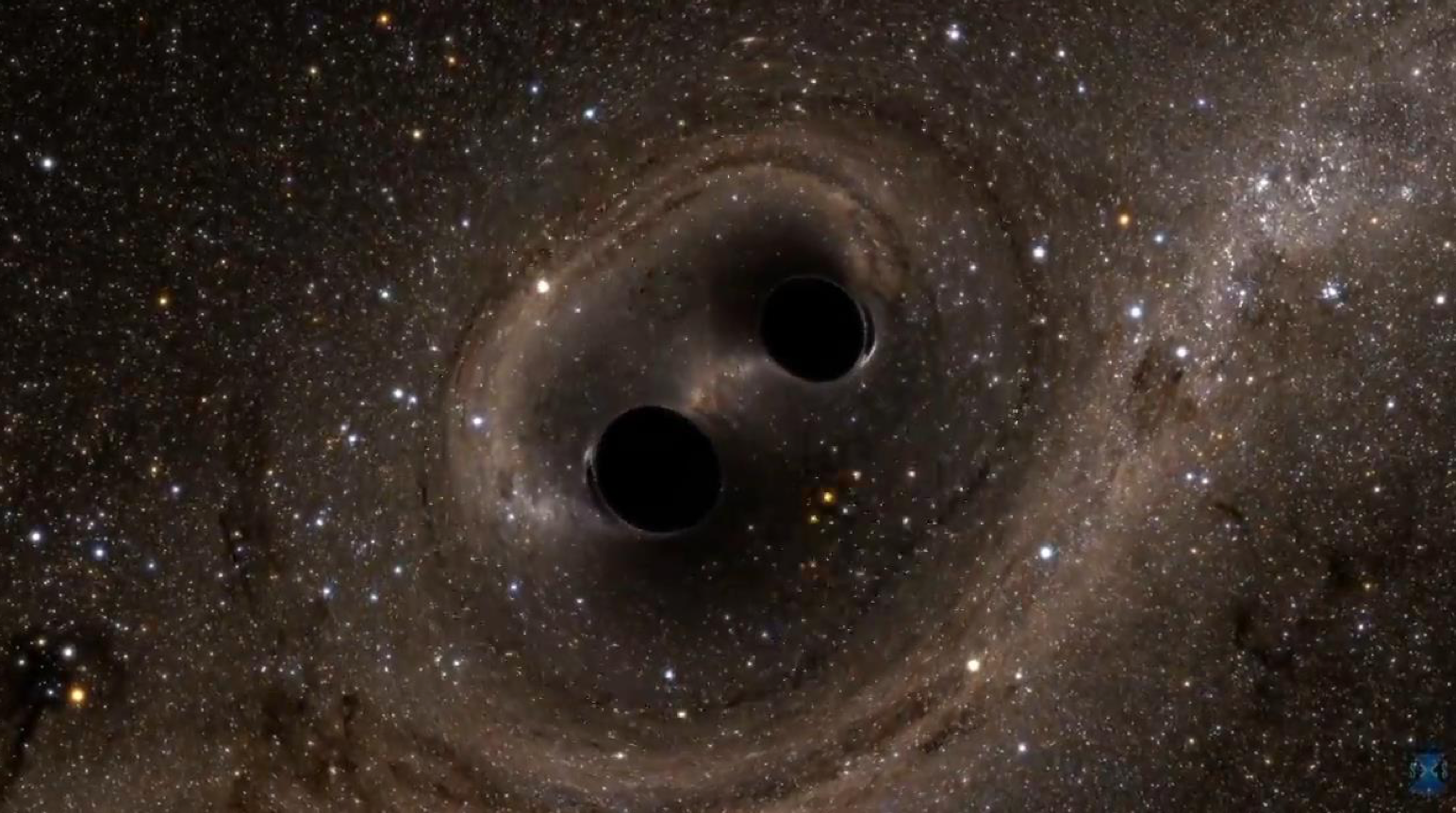
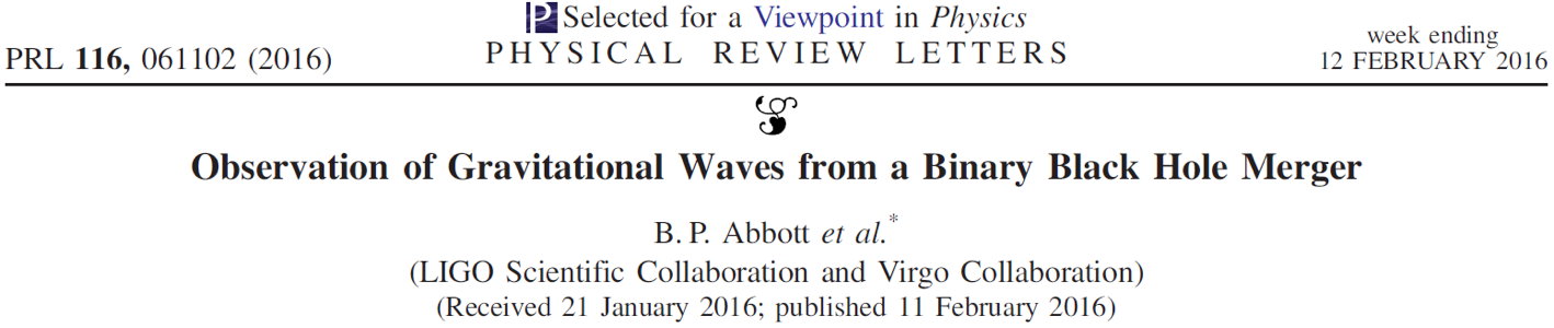
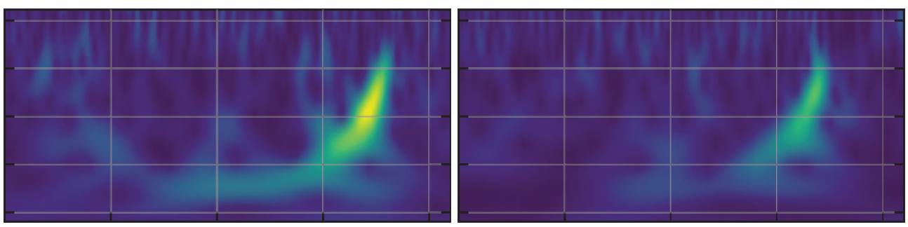
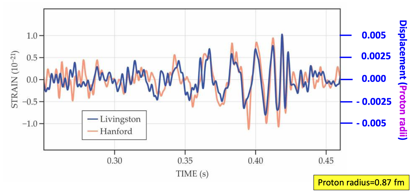
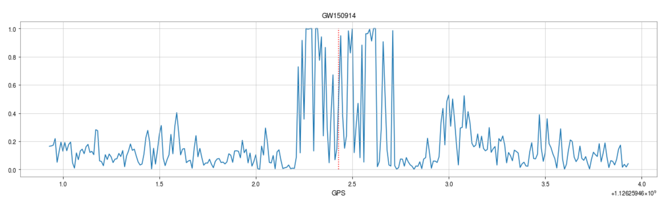
Event GW150914
Chirp-signal from gravitational waves from two coalescing black holes were observed with the LIGO detectors by the LIGO-Virgo Consortium on September 14, 2015
Background
Background
Event GW150914
Chirp-signal from gravitational waves from two coalescing black holes were observed with the LIGO detectors by the LIGO-Virgo Consortium on September 14, 2015
Background
Event GW150914
Chirp-signal from gravitational waves from two coalescing black holes were observed with the LIGO detectors by the LIGO-Virgo Consortium on September 14, 2015
Background
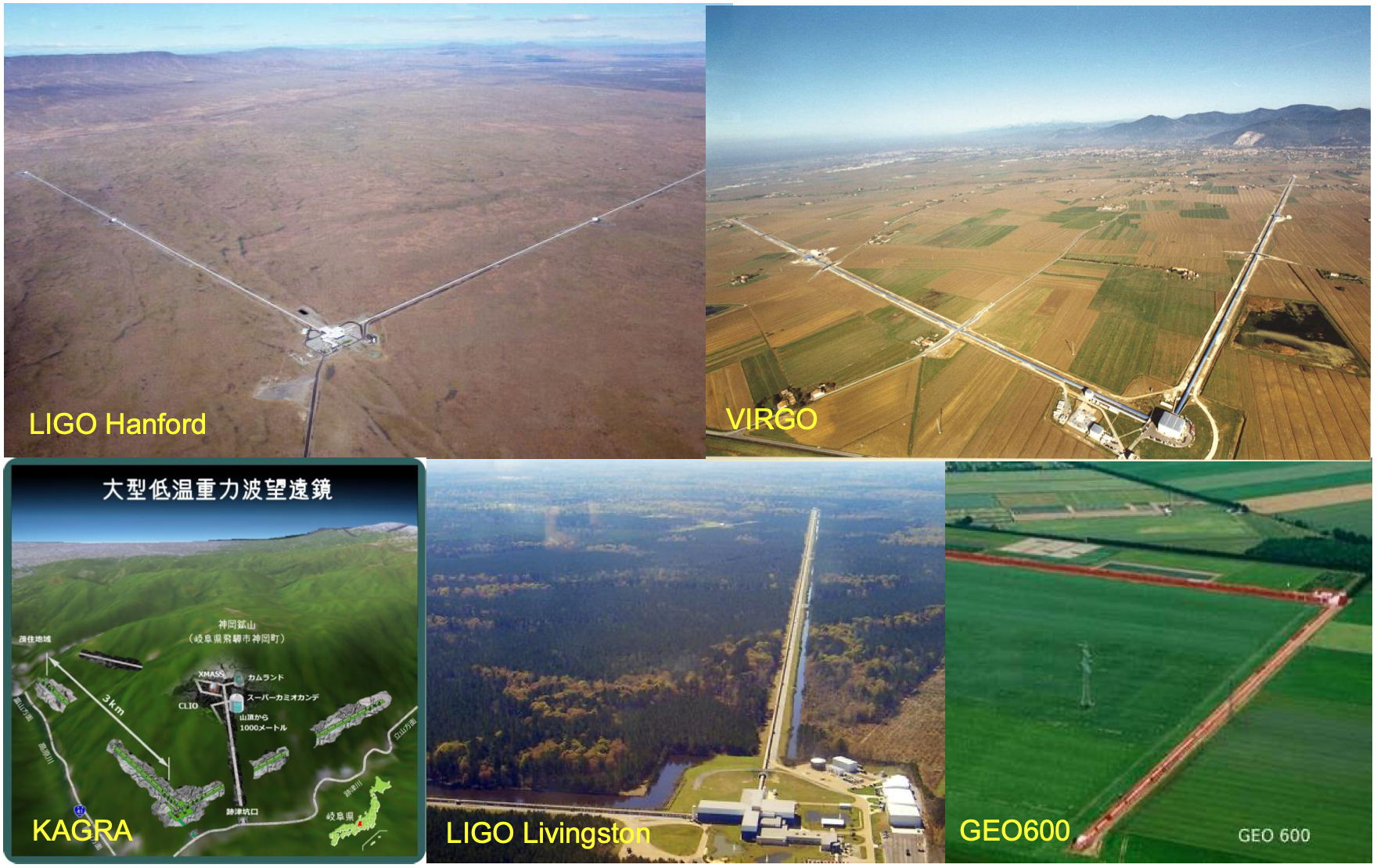
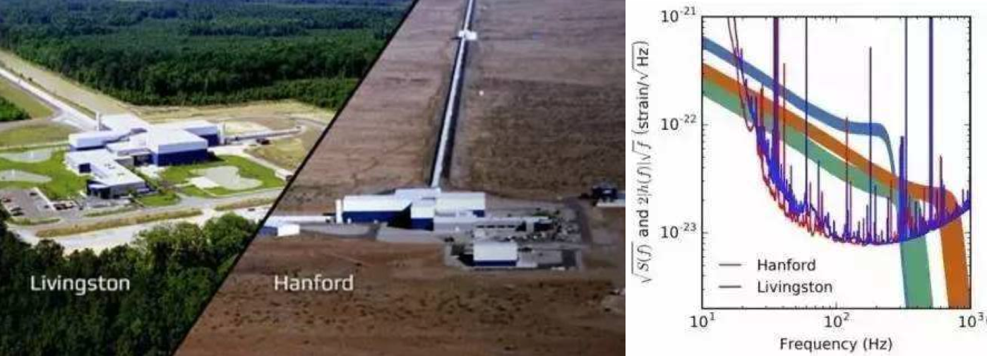
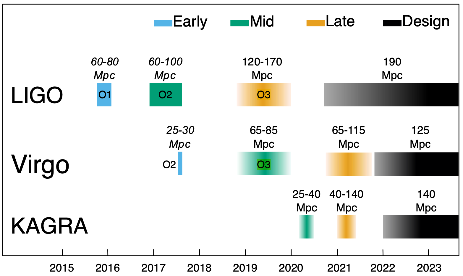
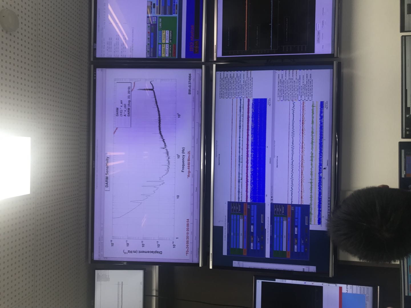
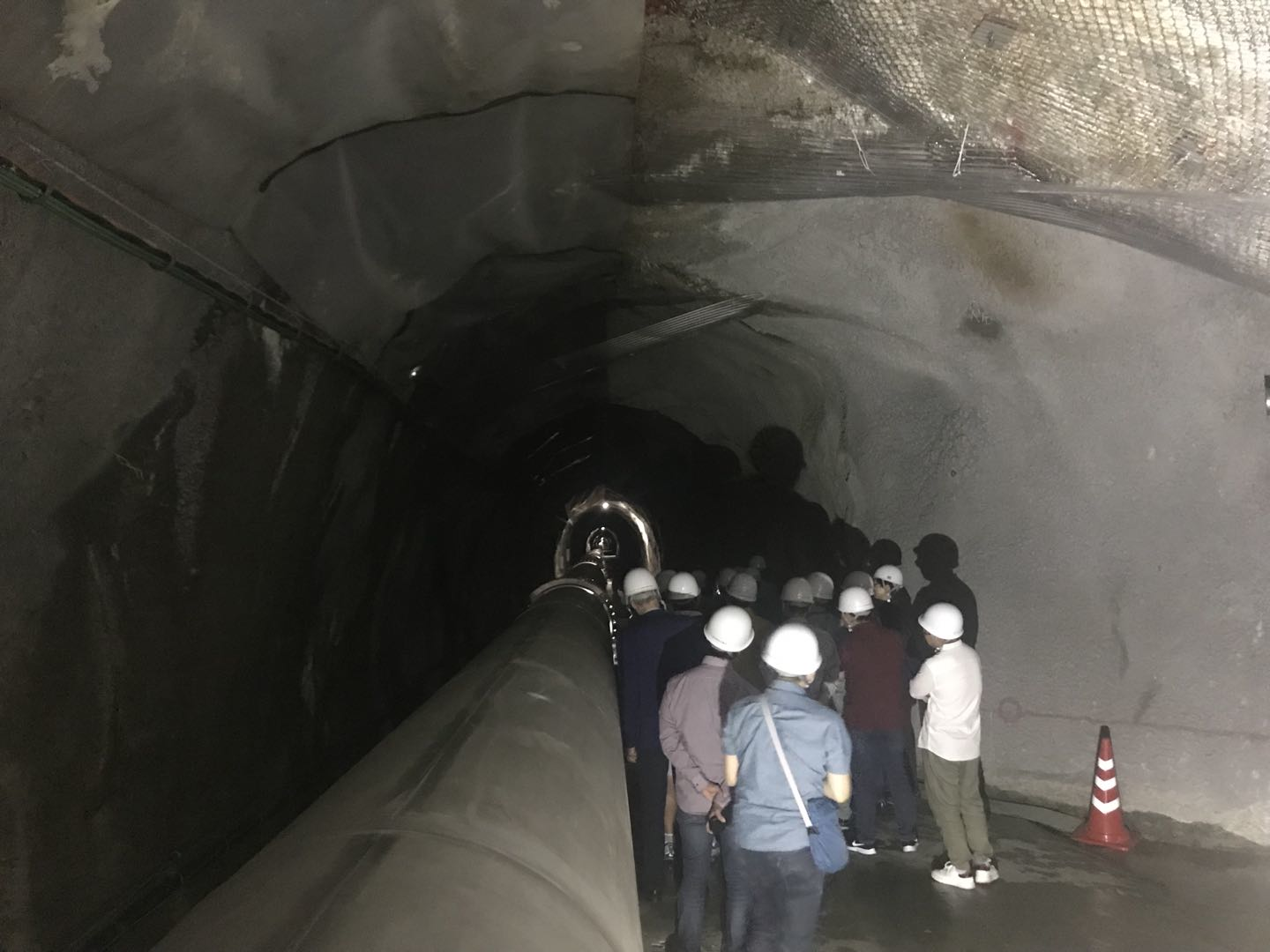
Laser interferometer detectors
Background
Laser interferometer detectors
Observation run O1:September 12, 2015 - January 19, 2016
B. P. Abbott et al., Prospects for Observing and Localizing Gravitational-Wave Transients with Advanced LIGO, Advanced Virgo and KAGRA, 2016, Living Rev. Relativity 19
Abbott et al, PRX 6, 041015 (2016)
Background
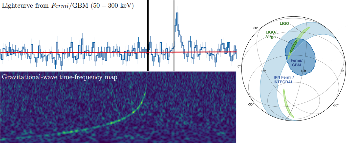
Multi-messenger astrophysics(多信使天文学)
曹周键. 从引力波探测到包含引力波的多信使天文学[J]. 大学物理, 2018, 37(2).
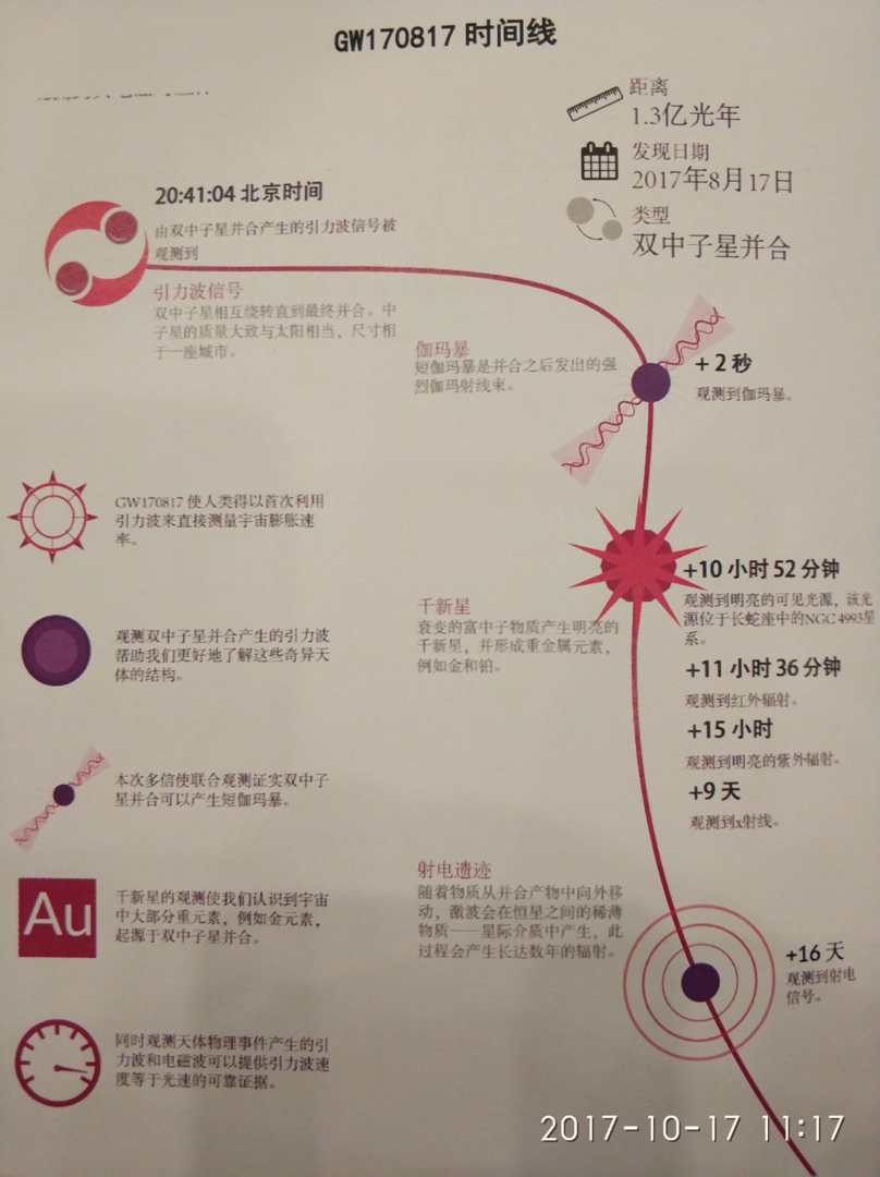
Event GW170817(首例双中子星合并事件)
LIGO and Virgo make first detection of gravitational waves produced by colliding neutron stars Discovery marks first cosmic event observed in both gravitational waves and light.
Background
Multi-messenger astrophysics(多信使天文学)
曹周键. 从引力波探测到包含引力波的多信使天文学[J]. 大学物理, 2018, 37(2).
Objective
2010 Class. Quantum Grav. 27 084005
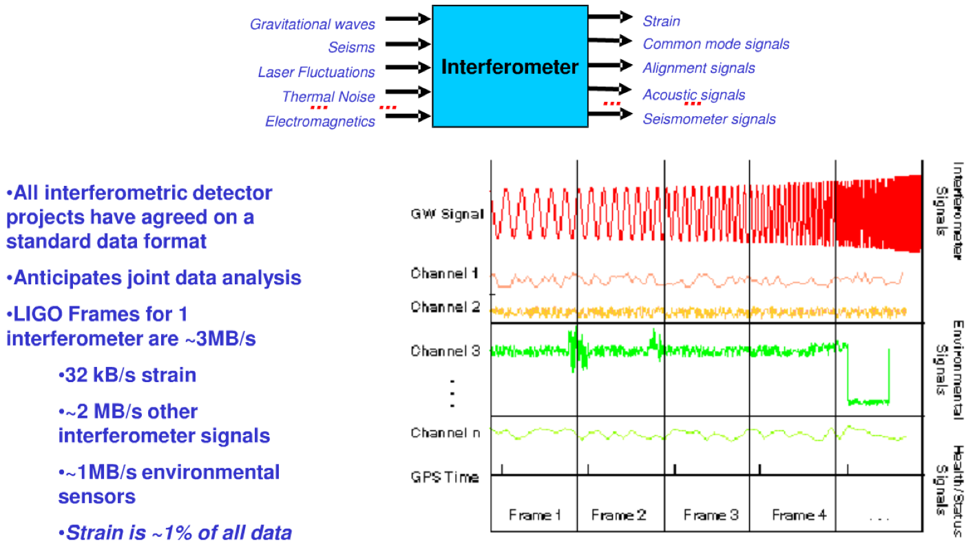
Data analysis
Basic of Data Analysis
Data analysis
Basic of Data Analysis
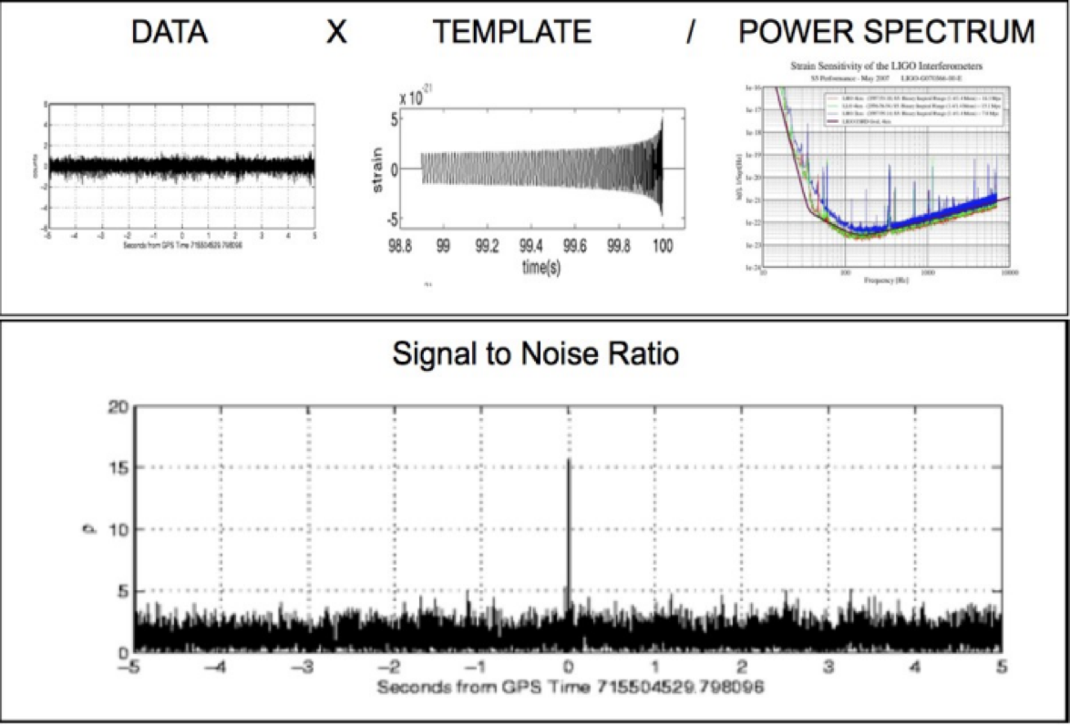
Data analysis and Matched-filtering techniques
Basic of Data Analysis
Data analysis and Matched-filtering techniques
Basic of Data Analysis
Data analysis and Matched-filtering techniques
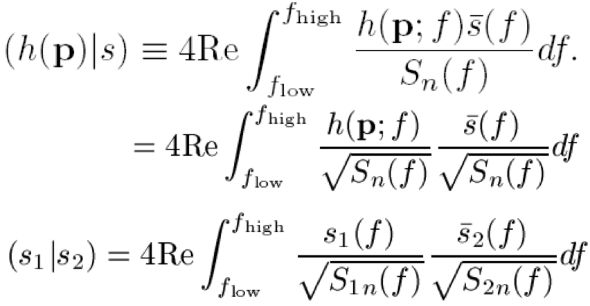
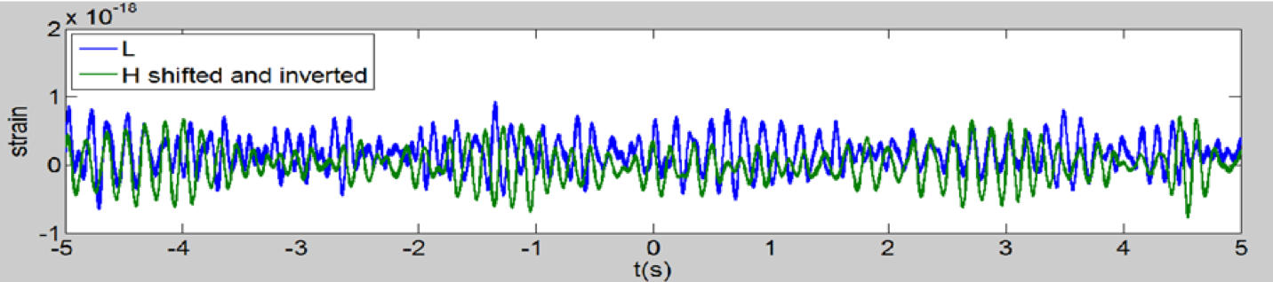
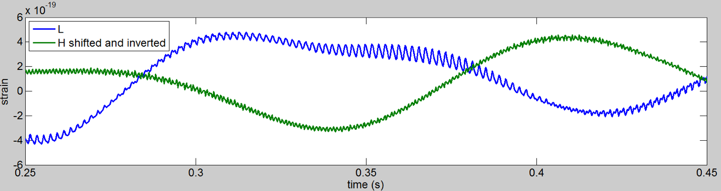
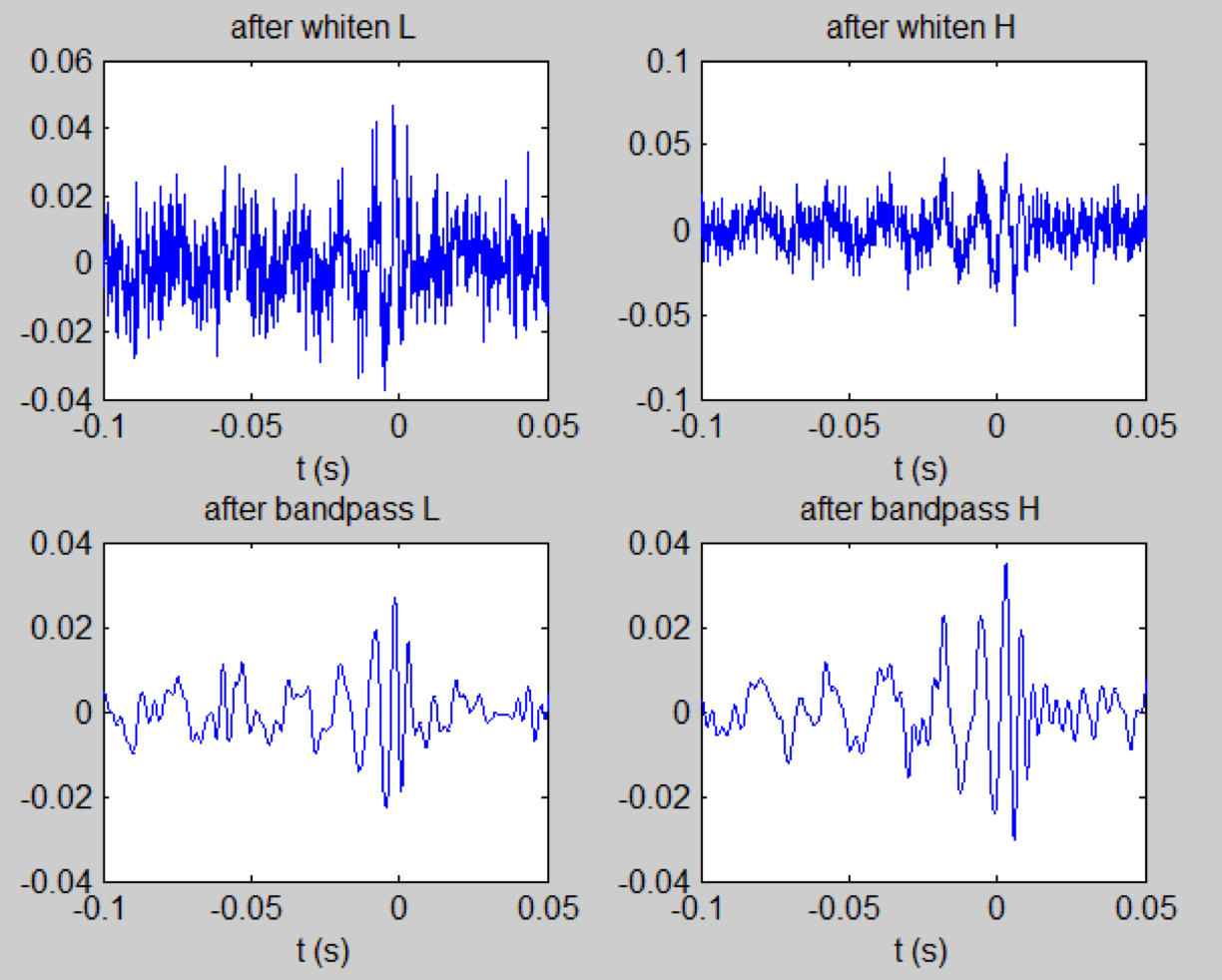
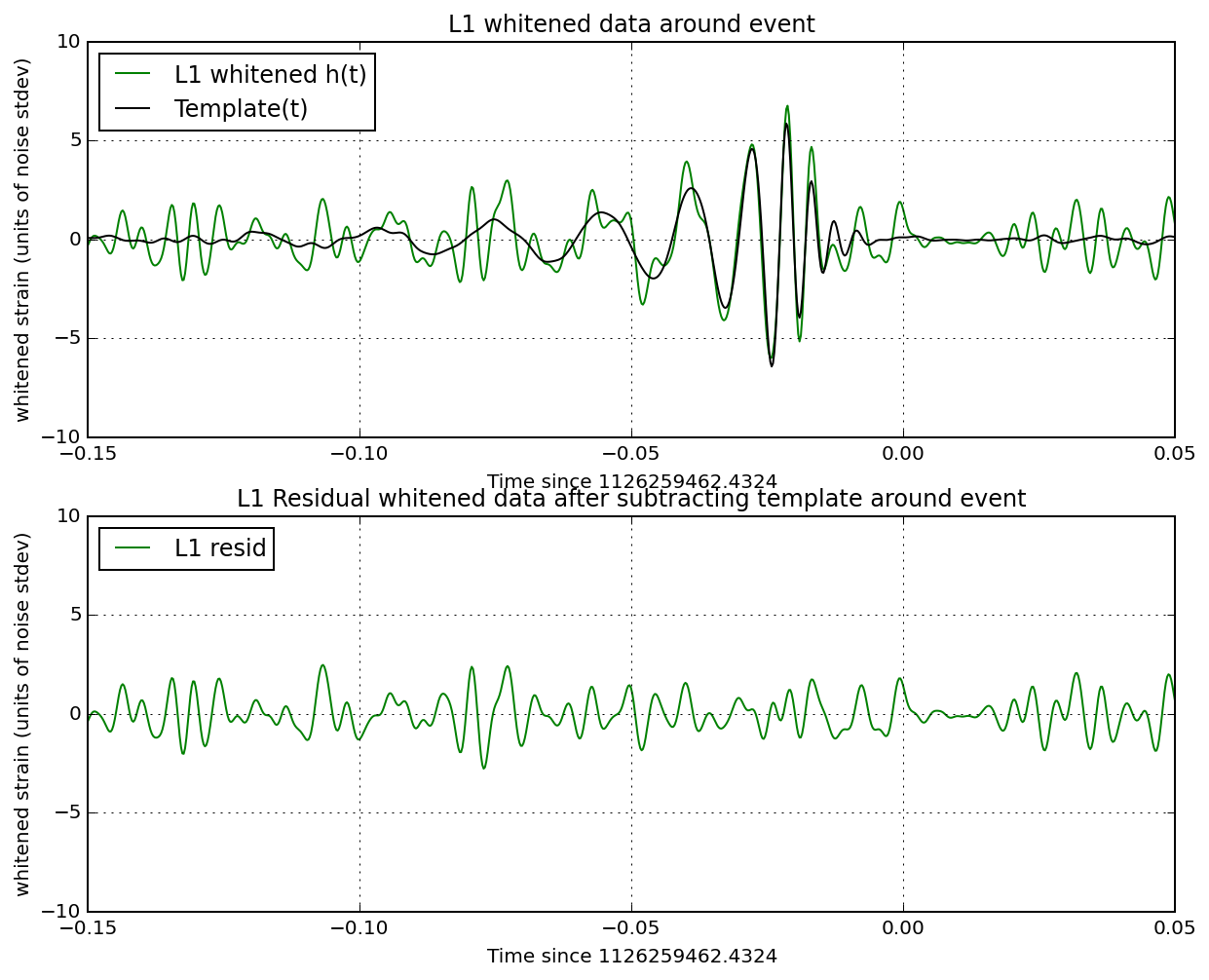
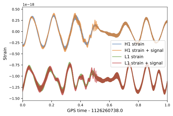
Whitening and filtering
Basic of Data Analysis
Data analysis and Matched-filtering techniques
Whitening and filtering
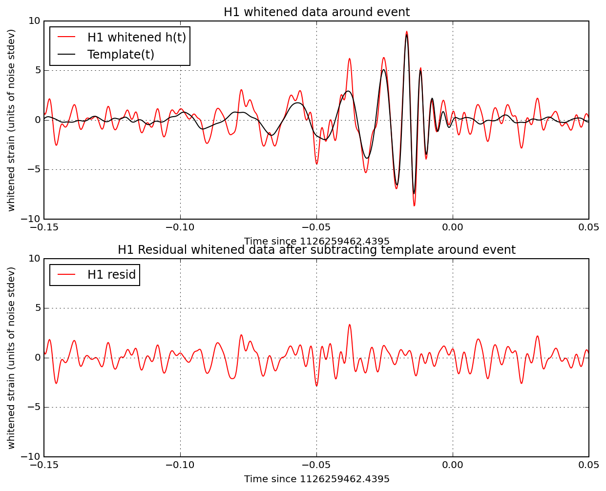
Basic of Data Analysis
Data analysis and Matched-filtering techniques
Whitening and filtering
Basic of Data Analysis
Data analysis and Matched-filtering techniques
Whitening and filtering
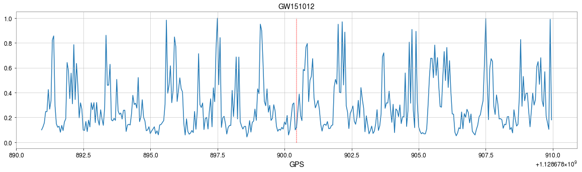
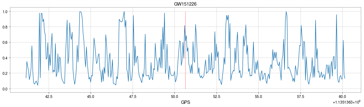
https://www.gw-openscience.org
Basic of Data Analysis
Data analysis and Matched-filtering techniques
Whitening and filtering
https://www.gw-openscience.org
Basic of Data Analysis
Solution:
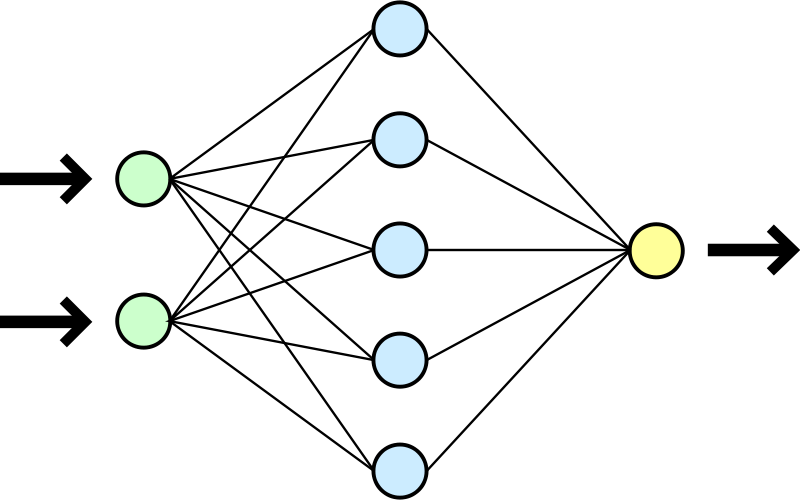
Machine Learning / Deep Learning
Map / Algorithm
Input
Output
A number
A sequence
Yes or No
Our model / network
Classification
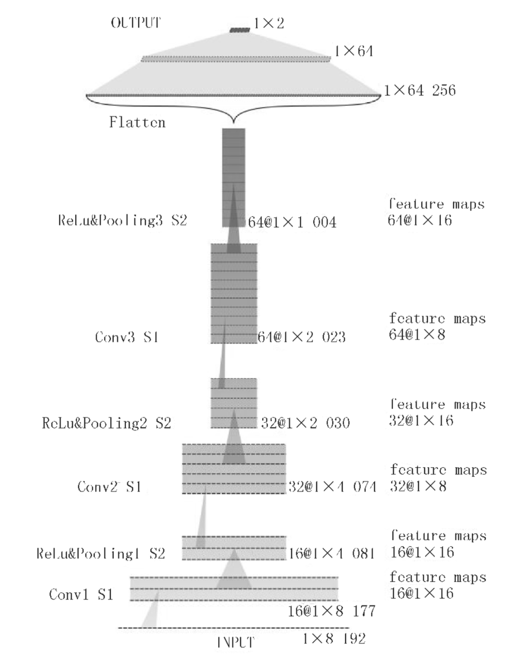
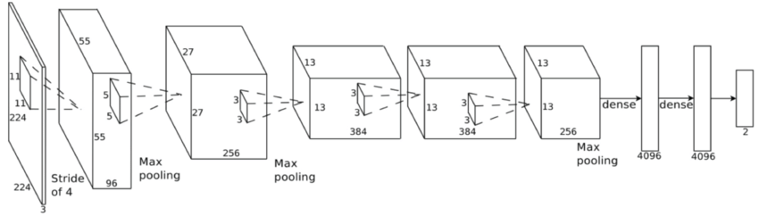
Convolutional neural network (ConvNet or CNN)
Feature extraction
Krizhevsky, A., Sutskever, I., & Hinton, G. E. (2012)
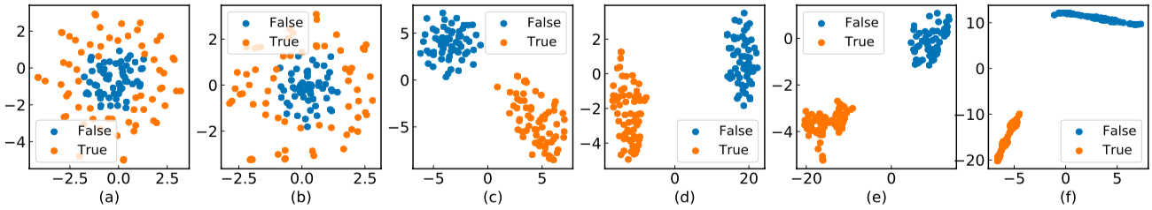
Visualization for the high-dimensional feature maps of learned network in layers for bi-class using t-SNE.
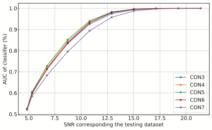
Effect of the number of the convolutional layers on signal recognizing accuracy.
Marginal!
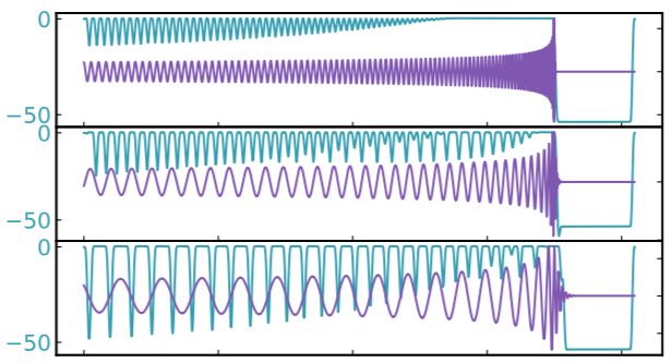
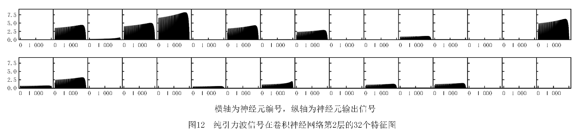
Visualization of the top activation on average at the \(n\)th layer projected back to time domain using the deconvolutional network approach
Visualization of the top activation on average at the \(n\)th layer projected back to time domain using the deconvolutional network approach
Occlusion Sensitivity
Peak of GW!
Occlusion Sensitivity
Peak of GW!
A specific design of the architecture is needed.
[as Timothy D. Gebhard et al. (2019)]
Motivation
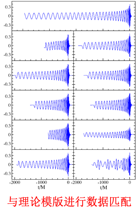
Matched-filtering in time domain
Matched-filtering ConvNet
Matched-filtering (cross-correlation with the templates) can be regarded as a convolutional layer with a set of predefined kernels.
Motivation
Motivation
Is it matched-filtering?
Matched-filtering (cross-correlation with the templates) can be regarded as a convolutional layer with a set of predefined kernels.
Frequency domain
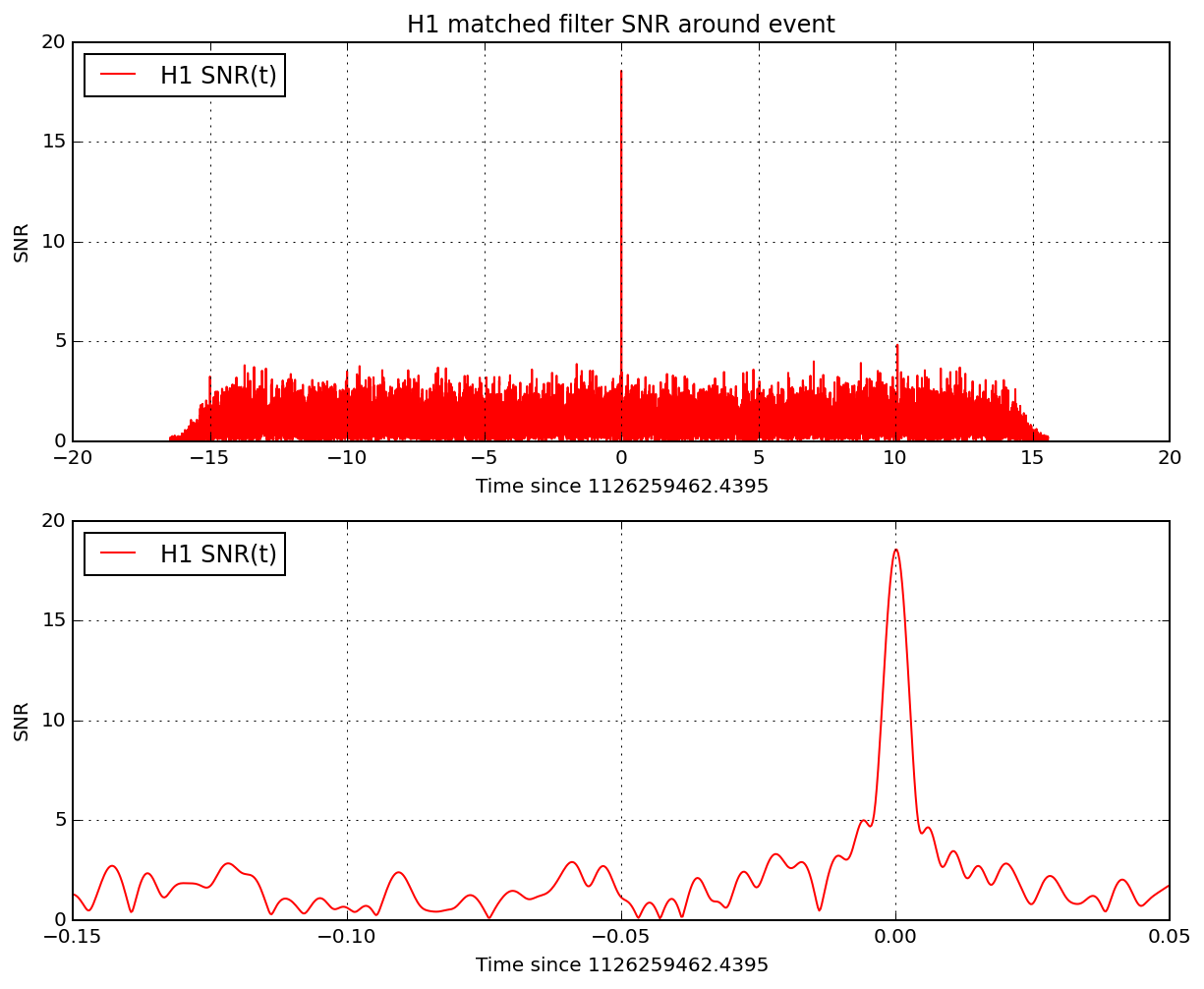
Matched-filtering in time domain
The square of matched-filtering SNR for a given data \(d(t) = n(t)+h(t)\):
The square of matched-filtering SNR for a given data \(d(t) = n(t)+h(t)\):
Matched-filtering in time domain
\(S_n(|f|)\) is the one-sided average PSD of \(d(t)\)
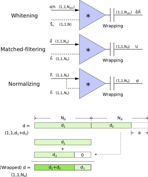
(whitening)
where
Time domain
Frequency domain
(normalizing)
(matched-filtering)
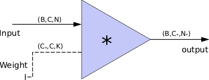
(A schematic illustration for a unit of convolution layer)
\(S_n(|f|)\) is the one-sided average PSD of \(d(t)\)
The square of matched-filtering SNR for a given data \(d(t) = n(t)+h(t)\):
Matched-filtering in time domain
(whitening)
where
(normalizing)
(matched-filtering)
Time domain
FYI: \(N_\ast = \lfloor(N-K+2P)/S\rfloor+1\)
In the 1-D convolution (\(*\)), given input data with shape [batch size, channel, length] :
Wrapping (like the pooling layer)
\(S_n(|f|)\) is the one-sided average PSD of \(d(t)\)
The square of matched-filtering SNR for a given data \(d(t) = n(t)+h(t)\):
Matched-filtering in time domain
(whitening)
where
(normalizing)
(matched-filtering)
Time domain
\(\bar{S_n}(t)\)
Architechture
Architechture
In the meanwhile, we can obtain the optimal time \(N_0\) (relative to the input) of feature response of matching by recording the location of the maxima value corresponding to the optimal template \(C_0\)
\(\bar{S_n}(t)\)
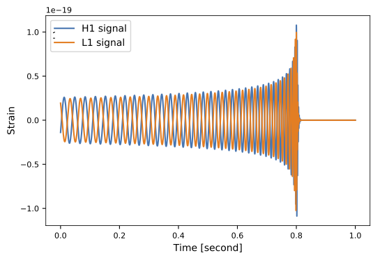
62.50M⊙ + 57.50M⊙ (\(\rho_{amp}=0.5\))
(In preprint)
FYI: sampling rate = 4096Hz
| template | waveform (train/test) | |
|---|---|---|
| Number | 35 | 1610 |
| Length (s) | 1 | 5 |
| equal mass |
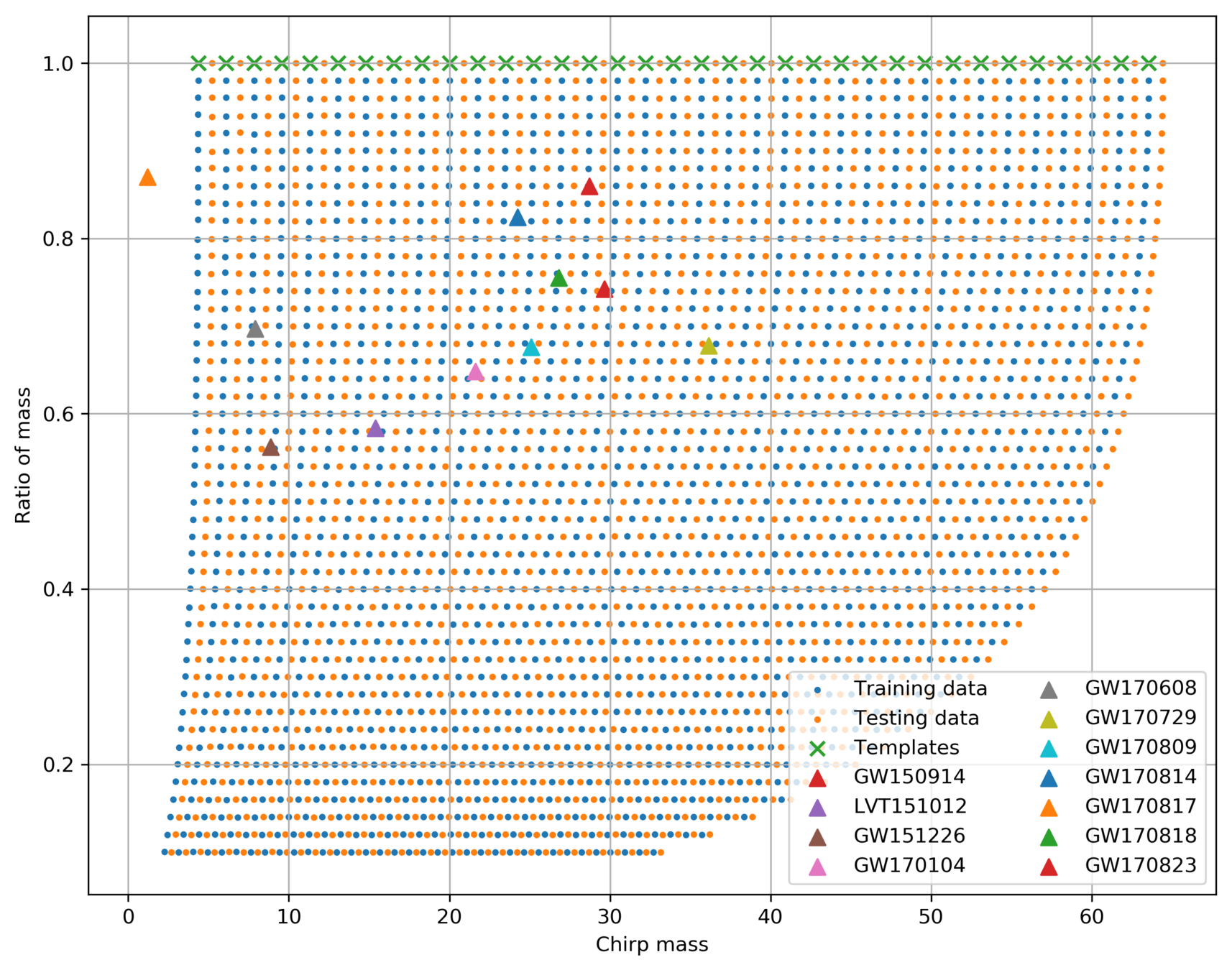
Dataset & Templates
FYI: sampling rate = 4096Hz
| template | waveform (train/test) | |
|---|---|---|
| Number | 35 | 1610 |
| Length (s) | 1 | 5 |
| equal mass |
(In preprint)
Dataset & Templates
(In preprint)
Probability
(sigmoid function)
Training Strategy
(In preprint)
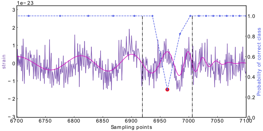
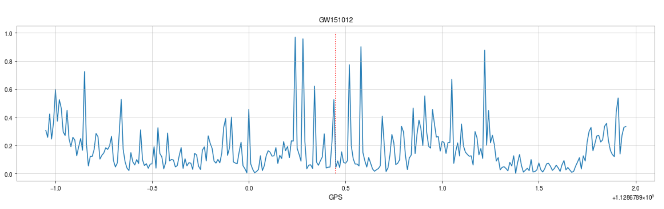
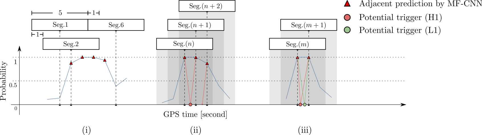
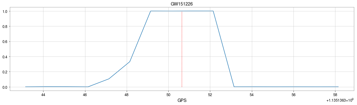
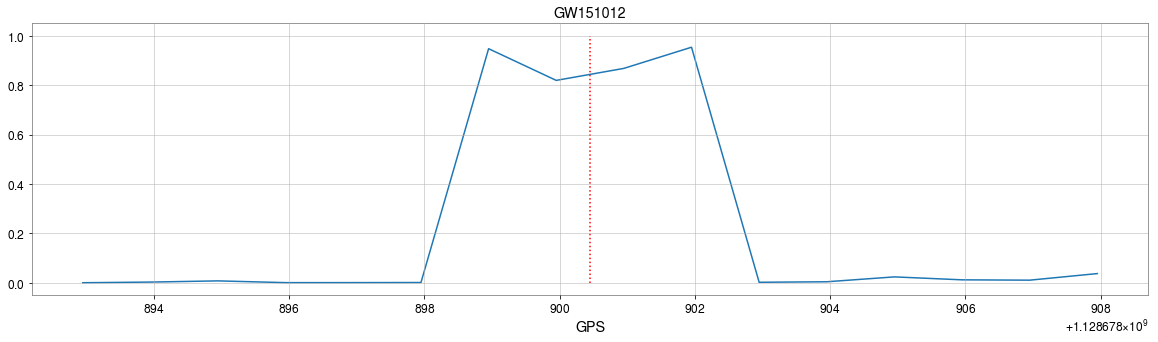
Search methodology
Input
(In preprint)
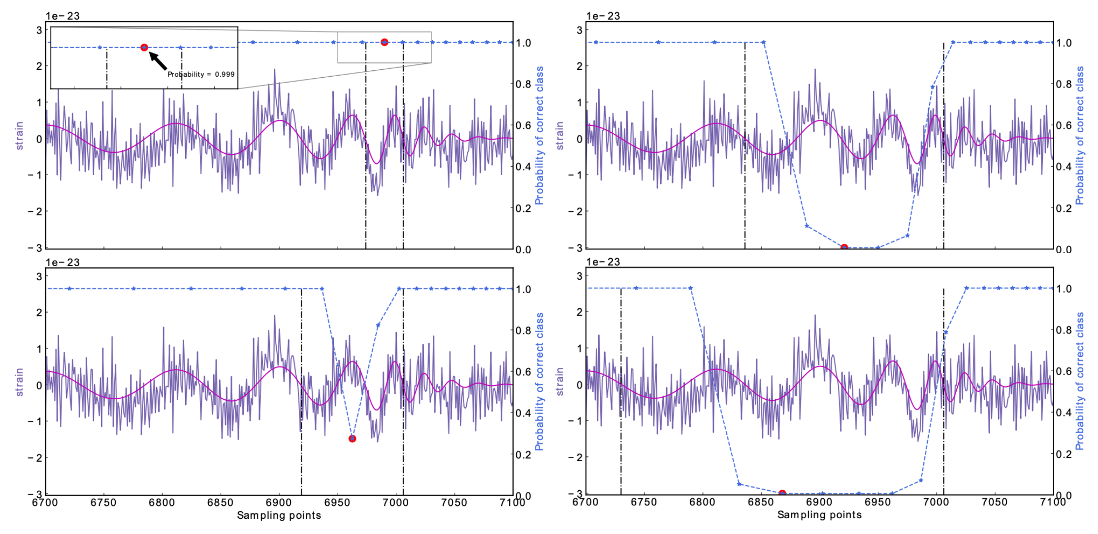
Search methodology
(In preprint)
(In preprint)
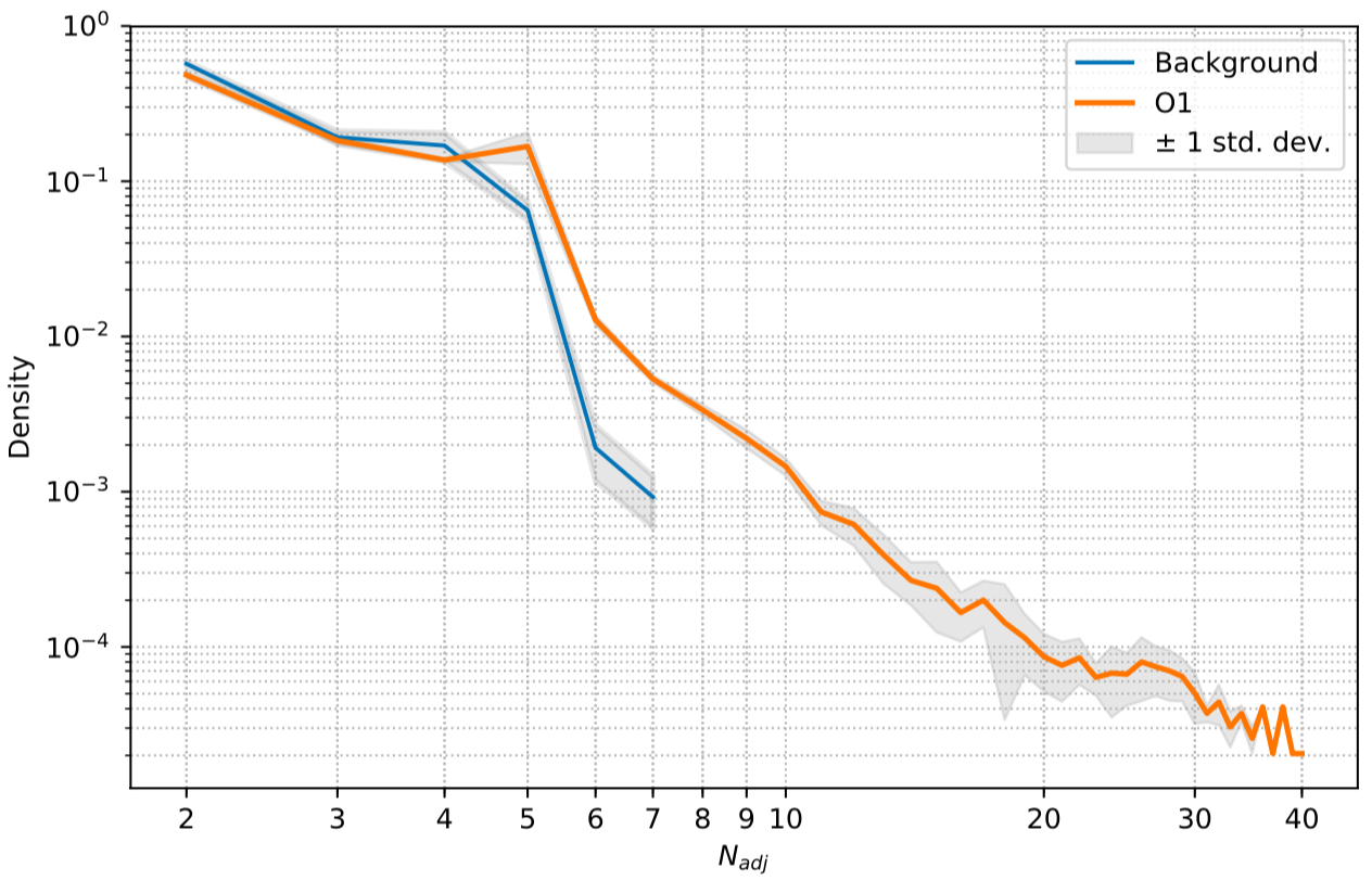
Number of Adjacent prediction
Population property on O1
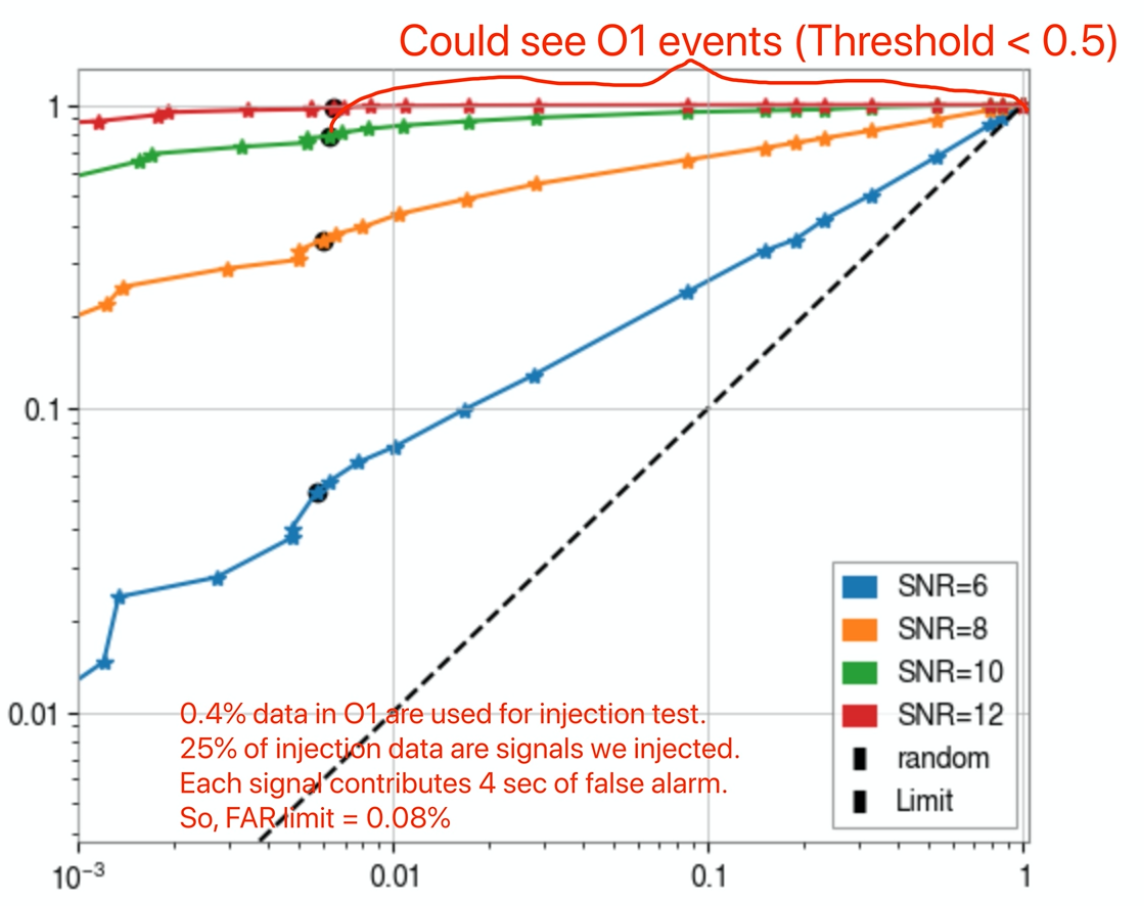
True Positive Rate
False Alarm Rate
(In preprint)
a bump at 5 adjacent predictions
Number of Adjacent prediction
Population property on O1
False Alarm Rate
True Positive Rate
(In preprint)
Some benefits from MF-CNN architechure
Simple configuration for GW data generation
Almost no data pre-processing
Easy parallel deployments, multiple detectors can be benefit a lot from this design
Some benefits from MF-CNN architechure
Simple configuration for GW data generation
Almost no data pre-processing
Easy parallel deployments, multiple detectors can be benefit a lot from this design
Thank you for your attention!
By He Wang
https://gdlab.ucas.ac.cn/index.php/zh-CN/xsbg-2/2907-2020-01-08-00-47-20 (Jan 10th, 2020)


