Support Vector Machine

Content

Introduction

What is a classification analysis?

What is a Support Vector and what is SVM?

How Svm classifier Works?

Examples of SVM boundaries

SVM Applications

Example (Python and scikit-learn)

Fisher’s classic 1936 paper (Iris flower)

Pros and Cons

Introduction

Let’s consider an example to understand these concepts. We have a population composed of 50%-50% Males and Females. Using a sample of this population, you want to create some set of rules which will guide us the gender class for rest of the population.

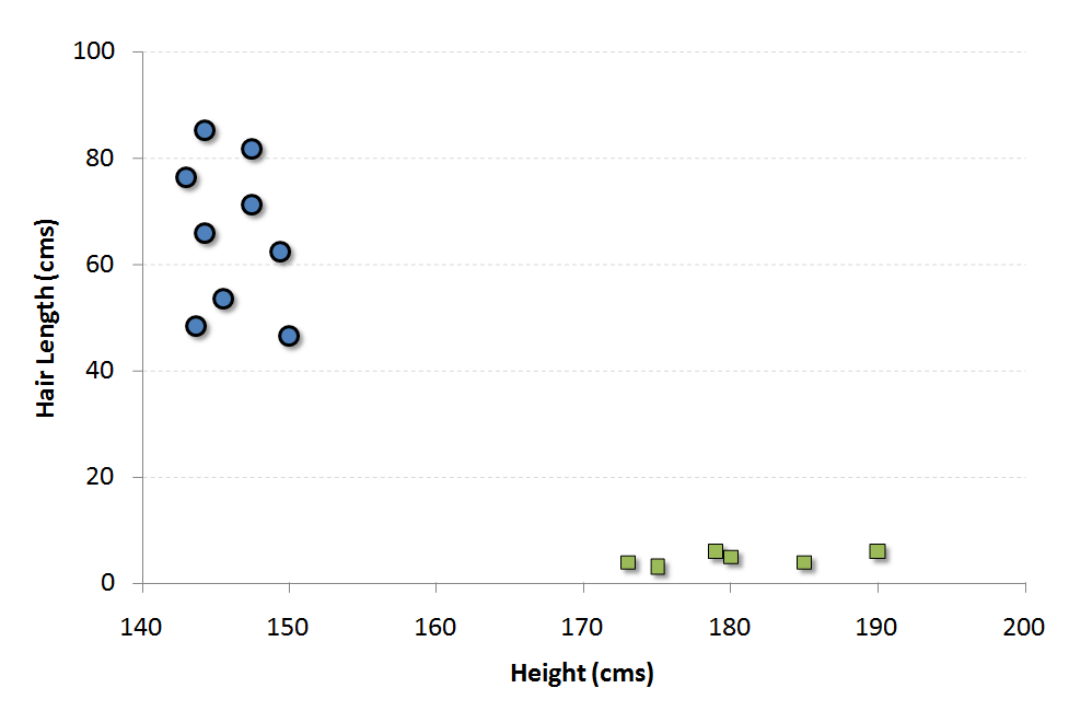
The blue circles in the plot represent females and green squares represents male. A few expected insights from the graph are : 1. Males in our population have a higher average height. 2. Females in our population have longer scalp hairs.

Support Vectors are simply the co-ordinates of individual observation.

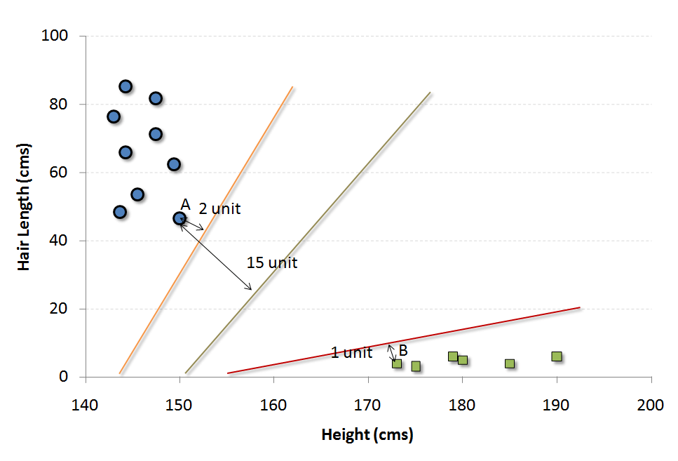
The easiest way to interpret the objective function in a SVM is to find the minimum distance of the frontier from closest support vector (this can belong to any class). we simply choose the frontier with the maximum distance (from the closest support vector). Out of the three shown frontiers, we see the black frontier is farthest from nearest support vector (i.e. 15 units).

Powerful technique for Classification, Regression & Outlier detection with an intuitive model

Supervised and Unsupervised learning

For a dataset consisting of features set and labels set, an SVM classifier builds a model to predict classes for new examples. It assigns new example/data points to one of the classes.

Linear SVM Classifier

Non-Linear SVM Classifier

It predicts a straight hyperplane dividing 2 classes. The primary focus while drawing the hyperplane is on maximizing the distance from hyperplane to the nearest data point of either class.

In the real world, our dataset is generally dispersed up to some extent.

In Non-Linear SVM Classification, data points plotted in a higher dimensional space.

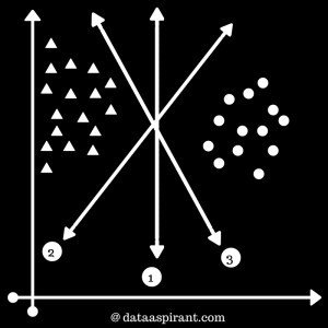
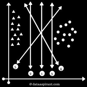
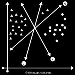
1st maximum margin

1st maximum margin

3 maximum margin

SVM will automatically ignore these triangles and select best-performing hyperplane. That is 1st

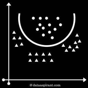
We can use different types of kernels like Radial Basis Function Kernel, Polynomial kernel etc. We have shown a decision boundary separating both the classes. This decision boundary resembles a parabola.

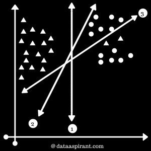
In the real world, you may find f ew values that correspond to extreme cases i.e, exceptions.These exceptions are known as Outliers. SVM have the capability to detect and ignore outliers.

SVMS are a byproduct of Neural Network. They are widely applied to pattern classification and regression problems. Here are some of its applications:

      * Facial expression classification: SVMs can be used to classify facial expressions. It uses statistical models of shape and SVMs.

    *Speech recognition: SVMs are used to accept keywords and reject non-keywords them and build a model to recognize speech.

*Handwritten digit recognition: Support vector classifiers can be applied to the recognition of isolated handwritten digits optically scanned.

     *Text Categorization: In information retrieval and then categorization of data using labels can be done by SVM.

sklearn.svm.SVC(C=1.0, kernel='rbf', degree=3, gamma=0.0, coef0=0.0, shrinking=True, 
probability=False,tol=0.001, cache_size=200, class_weight=None, verbose=False, max_iter=-1, 
random_state=None)

//parameters having higher impact on model performance, “kernel”, “gamma” and “C”

http://scikit-learn.org/stable/modules/generated/sklearn.svm.SVC.html

The 4 features are

SepalLengthCm
SepalWidthCm
PetalLengthCm
PetalWidthCm
 

The target class

The flower species type is the target class and it having 3 types

Setosa
Versicolor
Virginica

The idea of implementing svm classifier in Python is to use the iris features to train an svm classifier and use the trained svm model to predict the Iris species type.

# Required Packages
from sklearn import datasets		# To Get iris dataset
from sklearn import svm    			# To fit the svm classifier
import numpy as np
import matplotlib.pyplot as plt            # To visuvalizing the data

# import iris data to model Svm classifier
iris_dataset = datasets.load_iris()

print "Iris data set Description :: ", iris_dataset['DESCR']
print "Iris feature data :: ", iris_dataset['data']
print "Iris target :: ", iris_dataset['target']

def visuvalize_sepal_data():
	iris = datasets.load_iris()
	X = iris.data[:, :2]  # we only take the first two features.
	y = iris.target
	plt.scatter(X[:, 0], X[:, 1], c=y, cmap=plt.cm.coolwarm)
	plt.xlabel('Sepal length')
	plt.ylabel('Sepal width')
	plt.title('Sepal Width & Length')
	plt.show()

visuvalize_sepal_data()

Program 1

To visualize the Sepal length, width and corresponding target classes we can create a function with name visuvalize_sepal_data. At the beginning, we are loading the iris dataset to iris variable. Next, we are storing the first 2 features in iris dataset which are sepal length and sepal width to variable x. Then we are storing the corresponding target values in variable y.

# Required Packages
from sklearn import datasets		# To Get iris dataset
from sklearn import svm    			# To fit the svm classifier
import numpy as np
import matplotlib.pyplot as plt            # To visuvalizing the data

# import iris data to model Svm classifier
iris_dataset = datasets.load_iris()

print "Iris data set Description :: ", iris_dataset['DESCR']
print "Iris feature data :: ", iris_dataset['data']
print "Iris target :: ", iris_dataset['target']

def visuvalize_petal_data():
	iris = datasets.load_iris()
	X = iris.data[:, 2:]  # we only take the last two features.
	y = iris.target
	plt.scatter(X[:, 0], X[:, 1], c=y, cmap=plt.cm.coolwarm)
	plt.xlabel('Petal length')
	plt.ylabel('Petal width')
	plt.title('Petal Width & Length')
	plt.show()

visuvalize_petal_data()

Program 2

As we have successfully visualized the behavior of target class (iris species type) with respect to Sepal length and width as well as with respect to Petal length and width. Now let’s model different kernel Svm classifier by considering only the Sepal features (Length and Width) and only the Petal features (Lenght and Width)

# Required Packages
from sklearn import datasets		# To Get iris dataset
from sklearn import svm    			# To fit the svm classifier
import numpy as np
import matplotlib.pyplot as plt            # To visuvalizing the data
# import iris data to model Svm classifier
iris_dataset = datasets.load_iris()

print "Iris data set Description :: ", iris_dataset['DESCR']
print "Iris feature data :: ", iris_dataset['data']
print "Iris target :: ", iris_dataset['target']

iris = datasets.load_iris()
X = iris.data[:, :2]  # we only take the Sepal two features.
y = iris.target
C = 1.0  # SVM regularization parameter

# SVC with linear kernel
svc = svm.SVC(kernel='linear', C=C).fit(X, y)
# LinearSVC (linear kernel)
lin_svc = svm.LinearSVC(C=C).fit(X, y)
# SVC with RBF kernel
rbf_svc = svm.SVC(kernel='rbf', gamma=0.7, C=C).fit(X, y)
# SVC with polynomial (degree 3) kernel
poly_svc = svm.SVC(kernel='poly', degree=3, C=C).fit(X, y)
################First
h = .02  # step size in the mesh

# create a mesh to plot in
x_min, x_max = X[:, 0].min() - 1, X[:, 0].max() + 1
y_min, y_max = X[:, 1].min() - 1, X[:, 1].max() + 1
xx, yy = np.meshgrid(np.arange(x_min, x_max, h),
	                     np.arange(y_min, y_max, h))
# title for the plots
titles = ['SVC with linear kernel',
	   'LinearSVC (linear kernel)',
	    'SVC with RBF kernel',
	    'SVC with polynomial (degree 3) kernel']

for i, clf in enumerate((svc, lin_svc, rbf_svc, poly_svc)):
	 # Plot the decision boundary. For that, we will assign a color to each
	 # point in the mesh [x_min, x_max]x[y_min, y_max].
	 plt.subplot(2, 2, i + 1)
	 plt.subplots_adjust(wspace=0.4, hspace=0.4)

	 Z = clf.predict(np.c_[xx.ravel(), yy.ravel()])

	 # Put the result into a color plot
	 Z = Z.reshape(xx.shape)
	 plt.contourf(xx, yy, Z, cmap=plt.cm.coolwarm, alpha=0.8)

	 # Plot also the training points
	 plt.scatter(X[:, 0], X[:, 1], c=y, cmap=plt.cm.coolwarm)
	 plt.xlabel('Sepal length')
	 plt.ylabel('Sepal width')
	 plt.xlim(xx.min(), xx.max())
	 plt.ylim(yy.min(), yy.max())
	 plt.xticks(())
	 plt.yticks(())
	 plt.title(titles[i])

plt.show()

Program 3

# Required Packages
from sklearn import datasets		# To Get iris dataset
from sklearn import svm    			# To fit the svm classifier
import numpy as np
import matplotlib.pyplot as plt            # To visuvalizing the data
# import iris data to model Svm classifier
iris_dataset = datasets.load_iris()

print "Iris data set Description :: ", iris_dataset['DESCR']
print "Iris feature data :: ", iris_dataset['data']
print "Iris target :: ", iris_dataset['target']

iris = datasets.load_iris()
X = iris.data[:, 2:]  # we only take the last two features.
y = iris.target
C = 1.0  # SVM regularization parameter

# SVC with linear kernel
svc = svm.SVC(kernel='linear', C=C).fit(X, y)
# LinearSVC (linear kernel)
lin_svc = svm.LinearSVC(C=C).fit(X, y)
# SVC with RBF kernel
rbf_svc = svm.SVC(kernel='rbf', gamma=0.7, C=C).fit(X, y)
# SVC with polynomial (degree 3) kernel
poly_svc = svm.SVC(kernel='poly', degree=3, C=C).fit(X, y)

h = .02  # step size in the mesh
# create a mesh to plot in
x_min, x_max = X[:, 0].min() - 1, X[:, 0].max() + 1
y_min, y_max = X[:, 1].min() - 1, X[:, 1].max() + 1
xx, yy = np.meshgrid(np.arange(x_min, x_max, h),
	            np.arange(y_min, y_max, h))
# title for the plots
titles = ['SVC with linear kernel',
	  'LinearSVC (linear kernel)',
	  'SVC with RBF kernel',
	  'SVC with polynomial (degree 3) kernel']

for i, clf in enumerate((svc, lin_svc, rbf_svc, poly_svc)):
    # Plot the decision boundary. For that, we will assign a color to each
    # point in the mesh [x_min, x_max]x[y_min, y_max].
    plt.subplot(2, 2, i + 1)
    plt.subplots_adjust(wspace=0.4, hspace=0.4)

    Z = clf.predict(np.c_[xx.ravel(), yy.ravel()])

    # Put the result into a color plot
    Z = Z.reshape(xx.shape)
    plt.contourf(xx, yy, Z, cmap=plt.cm.coolwarm, alpha=0.8)

    # Plot also the training points
    plt.scatter(X[:, 0], X[:, 1], c=y, cmap=plt.cm.coolwarm)
    plt.xlabel('Petal length')
    plt.ylabel('Petal width')
    plt.xlim(xx.min(), xx.max())
    plt.ylim(yy.min(), yy.max())
    plt.xticks(())
    plt.yticks(())
    plt.title(titles[i])

plt.show()

Program 4

• SVMs are effective when the number of features is quite large.

• It works effectively even if the number of features are greater than the number of samples.

• Non-Linear data can also be classified using customized hyperplanes built by using kernel trick.

• It is a robust model to solve prediction problems since it maximizes margin.

• The biggest limitation of Support Vector Machine is the choice of the kernel. The wrong choice of the kernel can lead to an increase in error percentage.

• With a greater number of samples, it starts giving poor performances.

• SVMs have good generalization performance but they can be extremely slow in the test phase.

• VMs have high algorithmic complexity and extensive memory requirements due to the use of quadratic programming.