Programming - Old
Spark Programming
Intro to Spark
Spark Programming
Intro to Spark
Spark started as a research project in the
UC Berkeley RAD Lab - later became AMPLab.
- 2009: Created, already 10-20x faster than MapReduce
-
2011: AMPLab added Berkeley Data Analytics Stack
- Shark (Hive on Spark), later replaced by Spark SQL
- Spark Streaming
- Mar, 2010: Open sourced under Apache 2.0
- June, 2013: Transferred to the Apache SF
- May, 2014: Spark 1.0 released
- July, 2016: Spark 2.0 released
- https://spark.apache.org/news/
Spark Programming
Intro to Spark
- Approaching 1 million lines of code
- Runs on the Java VM
- Mostly written in Scala
- Backporting key APIS to Java
- 1000+ Contributors
https://github.com/apache/spark/graphs/contributors - Hundreds of contributing companies
- Most active, big-data, open source project
Spark Programming
Intro to Spark
Spark Programming
Intro to Spark
Spark Programming
Intro to Spark
The Driver
Spark Programming
Intro to Spark
The Cluster Manager
Spark Programming
Intro to Spark
The Executor
Spark Programming
Intro to Spark
Driver & Executor
Spark Programming
Who is Databricks
Spark Programming
Spark Core
Spark Programming
RDDs
Spark Programming
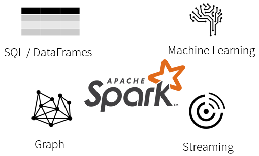
DataFrames/Datasets
Spark Programming
Spark SQL
Spark Programming
GraphX/GraphFrames
Spark Programming
Spark Streaming
Spark Programming
Intro to Spark ML
Spark Programming
Intro to Spark ML
ML vs MLLib
Spark Programming
Natural Language
Processing Lab
Spark Programming
Natural Language Processing Lab
Business Questions
- What percentage of Wikipedia articles were edited in the past month?
- How many of the 1 million articles were last edited by ClueBot NG, an anti-vandalism bot?
- Which user in the 1 million articles was the last editor of the most articles?
- Can you display the titles of the articles in Wikipedia that contain a particular word?
- Can you extract out all of the words from the Wikipedia articles? (bag of words)
- What are the top 15 most common words in the English language?
- After removing stop words, what are the top 10 most common words?
- How many distinct/unique words are in noStopWordsListDF?
Spark Programming
Natural Language Processing Lab
Accomplishments
- Work with 2% of the sum of all human knowledge!
- Work with some of the Spark ML's Feature Extraction API
Spark Programming
TF-IDF & K-Means Lab
Spark Programming
TF-IDF & K-Means Lab
- one
- two
- three
Spark Programming
Power Plant Labs
Spark Programming
Power Plant Labs
-
We are trying to predict power output given a set of readings from various sensors in a gas-fired power generation plant.
-
Power generation is a complex process, and understanding and predicting power output is an important element in managing a plant and its connection to the power grid
- More information about Peaker or Peaking Power Plants can be found on Wikipedia https://en.wikipedia.org/wiki/Peaking_power_plant
Spark Programming
Power Plant Labs
-
The ML task is regression since the label (or target) we are trying to predict is numeric.
- The example data is provided by UCI at UCI Machine Learning Repository Combined Cycle Power Plant Data Set
- This lab will only work with Spark 1.4 or later
val v = sc.version.replace(".", "").toInt >= 140
require(v, "Spark 1.4.0+ is required for this lab.")
Spark Programming
Power Plant Labs
Step 1: Business Understanding
-
The first step in any machine learning task is to understand the business need.
-
As described in the overview we are trying to predict power output given a set of readings from various sensors in a gas-fired power generation plant.
-
The problem is a regression problem since the label (or target) we are trying to predict is numeric
Spark Programming
Power Plant Labs
Step 2: Download Your Data
- The Easy Way: download all five files
- The Hard Way
- Data the Download Folder from the UCI Machine Learning Repository Combined Cycle Power Plant Data Set
https://archive.ics.uci.edu/ml/datasets/Combined+Cycle+Power+Plant - Save each tab as a seperate text file - TSV tends to be more consistent than CSV.
- Data the Download Folder from the UCI Machine Learning Repository Combined Cycle Power Plant Data Set
Spark Programming
Power Plant Labs
Step 3: Upload Your Data
- Select the Tables icon.
- Click on + Create Table
- Set the Data Source to File
- Add all five files at once (drag & drop)
- Click Preview Table
- Set Table name to power_plant
- Set File type to CSV
- Set Column Delimiter to \t
- Check First row is header
- Change all five column types to Double
- Click Create Table
Spark Programming
Power Plant Labs
Step 4: Explore Your Data
- Quick select from the power_plant
- Let's take a look at the schmea
- What are we looking at?
- AT = Atmospheric Temperature in C
- V = Exhaust Vacuum Speed
- AP = Atmospheric Pressure
- RH = Relative Humidity
- PE = Power Output (our label or target)
- Review some of the table's basic stats
%sql
SELECT * FROM power_plant
%sql
desc power_plantvar tempDF = sqlContext.table("power_plant").describe()Spark Programming
Power Plant Labs
Step 5: Look for correlations
- This will affect which model we use.
- If the feature and label are linearly correlated, a linear model like Linear Regression can do well.
- If very non-linear, more complex modles such as Decision Trees might be better.
Spark Programming
Power Plant Labs
Step 5a: Temperature vs Power
- Quick select statement to view the data
- Create a scatter plot
- We can see a strong, linear correlation
%sql
select AT as Temperature, PE as Power from power_plant
Spark Programming
Power Plant Labs
Step 5b: Exhaust Vacuum vs Power
- Quick select statement to view the data
- Create a scatter plot
- Semi-linear, but not as strong as temperature
%sql
select V as ExhaustVacuum, PE as Power from power_plant;
Spark Programming
Power Plant Labs
Step 5c: Pressure vs Power
- Quick select statement to view the data
- Create a scatter plot
- Little to no linear correlation
%sql
select AP as Pressure, PE as Power from power_plant;
Spark Programming
Power Plant Labs
Step 5d: Humidity vs Power
- Quick select statement to view the data
- Create a scatter plot
- Little to no linear correlation
%sql
select RH as Humidity, PE as Power from power_plant;
Spark Programming
Power Plant Labs
Step 6: Prepare Our Data
- All the data is numeric so not much clean up
- We need to convert columns to Feature Vectors
- See org.apache.spark.ml.feature.VectorAssembler
import org.apache.spark.ml.feature.VectorAssembler

val dataset = sqlContext.table("power_plant")

val vectorizer = new VectorAssembler()
vectorizer.setInputCols(Array("AT", "V", "AP", "RH"))
vectorizer.setOutputCol("features")
Spark Programming
Power Plant Labs
Step 7: Linear Regression
- We saw one REALLY strong, linear correlation and a couple of other weak correlations.
- Let's start with a Linear Regression model
Spark Programming
Power Plant Labs
Step 7a: Setup Training Data
- Hold out 20% of our data for testing, 80% for modeling
// Create a 20/80 split
var Array(split20, split80) = dataset.randomSplit(Array(0.20, 0.80), 1800009193L)

// Cache our data
val testSet = split20.cache()
val trainingSet = split80.cache()

// materialize our caches
testSet.count()
trainingSet.count()
Spark Programming
Power Plant Labs
Step 7b: Create the Model
- Import our classes and create an new instance
- Let's see what parameters we can use
- Configure the model's parameters
import org.apache.spark.ml.regression.LinearRegression
import org.apache.spark.ml.regression.LinearRegressionModel
import org.apache.spark.ml.Pipeline

val lr = new LinearRegression()lr.explainParams()lr.setPredictionCol("Predicted_PE")
.setLabelCol("PE")
.setMaxIter(100)
.setRegParam(0.1)Spark Programming
Power Plant Labs
Step 7c: Setup the Pipeline
- Instantiate a new Pipeline
- Setup the pipeline with two sages
- The vectorizer
- The linear regression model lr
- Create the model by fitting the pipeline
with our training set
val lrPipeline = new Pipeline()lrPipeline.setStages(Array(vectorizer, lr))val lrModel = lrPipeline.fit(trainingSet)Spark Programming
Power Plant Labs
Step 8: Understanding Our Model
- Linear Regression is Simply a Line of best fit over the data that minimizes the square of the error
- given multiple input dimensions we can express each predictor as a line function of the form:
%[ y = a + b x_1 + b x_2 + b x_i ... ]%
where a is the intercept and b are the coefficients
- To express the coefficients of that line we can retrieve the Estimator stage from the PipelineModel and express the weights and the intercept for the function.
Spark Programming
Power Plant Labs
Step 8a: Compute the Equation
- We can get the intercept from the 2nd stage of the model
- Get the weights and the coefficients
- Construct the "equation" from a sorted set of coefficients
val lrm = lrModel.stages(1).asInstanceOf[LinearRegressionModel]
val intercept = lrm.intercept
val weights = lrModel.stages(1).asInstanceOf[LinearRegressionModel].weights.toArray
val featuresNoLabel = dataset.columns.filter(col => col != "PE")
val coefficents = sc.parallelize(weights).zip(sc.parallelize(featuresNoLabel))var equation = s"y = $intercept "
var variables = Array
coefficents.sortByKey().collect().foreach(x =>
{
val weight = Math.abs(x._1)
val name = x._2
val symbol = if (x._1 > 0) "+" else "-"
equation += (s" $symbol (${weight} * ${name})")
}
)
println("Linear Regression Equation: " + equation)Spark Programming
Power Plant Labs
Step 8b: Evaluating our Equation
- We have a strong correlation between atmospheric temperature and power output
- The other dimensions seem to have little to no correlation (we saw this in our scatter plots)
Spark Programming
Power Plant Labs
Step 9: Some Real Predictions
- Using the model, lrModel, transfor our testSet.
- We can see that our predictions are pretty good,
but how good are they?
val predictionsAndLabels = lrModel.transform(testSet)
val predictions = predictionsAndLabels.select("AT", "V", "AP", "RH", "PE", "Predicted_PE")
display(predictions)
Spark Programming
Power Plant Labs
Step 10a: Validating our Results
- Let's start by preparing our results
- Create a RegressionMetrics from those results
- Print the results
- A good model will have...
- 68% of predictions within 1 RMSE
- 95% of predictions within 2 RMSE
val rowRDD = predictionsAndLabels.select("Predicted_PE", "PE").rdd
val results = rowRDD.map(r => (r(0).asInstanceOf[Double], r(1).asInstanceOf[Double]))
import org.apache.spark.mllib.evaluation.RegressionMetrics
val metrics = new RegressionMetrics(results)printf("Root Mean Squared Error: %s\n", metrics.rootMeanSquaredError)
printf("Explained Variance: %s\n", metrics.explainedVariance)
printf("R2: %s\n", metrics.r2)
println("="*40)Spark Programming
Power Plant Labs
Step 10b: Crunching the RMSE
- Calculate the residual error
- Using some simple SQL, we can generate our results
- Render the results as a pie chart
val tempDF = predictionsAndLabels.selectExpr(
  "PE",
  "Predicted_PE",
  "PE - Predicted_PE Residual_Error",
  s""" abs(PE - Predicted_PE) / ${metrics.rootMeanSquaredError} Within_RSME""")

tempDF.registerTempTable("Power_Plant_RMSE_Evaluation") // for later
display(tempDF)
%sql
SELECT ceiling(Within_RSME) as Within_RSME,
count(*) as count
from Power_Plant_RMSE_Evaluation
GROUP BY ceiling(Within_RSME)Spark Programming
Power Plant Labs
Step 11a: RE & CV
Let's try to make a better model by tuning over several parameters to see if we can get better results
- Add some imports
- Let's setup our evaluator class to judge the model based on the best root mean squared error
- Create our crossvalidator with 3 fold cross validation
import org.apache.spark.ml.tuning.{ParamGridBuilder, CrossValidator}
import org.apache.spark.ml.evaluation._
val regEval = new RegressionEvaluator()
regEval.setLabelCol("PE")
.setPredictionCol("Predicted_PE")
.setMetricName("rmse")val crossval = new CrossValidator()
crossval.setEstimator(lrPipeline)
crossval.setNumFolds(5)
crossval.setEvaluator(regEval)Spark Programming
Power Plant Labs
Step 11b: Create the Model
- Let's tune over our regularization
parameter from 0.01 to 0.10
- Create the model by fitting our training
set to our cross validator
val regParam = ((1 to 10) toArray).map(x => (x /100.0))

val paramGrid = new ParamGridBuilder()
  .addGrid(lr.regParam, regParam)
  .build()
crossval.setEstimatorParamMaps(paramGrid)
val cvModel = crossval.fit(trainingSet)Spark Programming
Power Plant Labs
Step 11c: Recompute RMSE
- Let's evaluate the result for tuning parameters and what our RMSE was versus our initial model
- Tuned & untuned are statistically identical
- Will another model such as Decision Tree work better?
val predictionsAndLabels = cvModel.transform(testSet)
val result = predictionsAndLabels
  .select("Predicted_PE", "PE").rdd
  .map(r => (r(0).asInstanceOf[Double], r(1).asInstanceOf[Double]))
val metrics = new RegressionMetrics(result)

printf(s"Root Mean Squared Error: %s\n", metrics.rootMeanSquaredError)
printf(s"Explained Variance: %s\n", metrics.explainedVariance)
printf(s"R2: %s\n", metrics.r2)
println("="*40)
Spark Programming
Power Plant Labs
Step 12a: Setup a Decision Tree Model
A Decision Tree creates a model based on splitting variables using a tree structure. We will first start with a single decision tree model.
import org.apache.spark.ml.regression.DecisionTreeRegressor

val dt = new DecisionTreeRegressor()
dt.setLabelCol("PE")
dt.setPredictionCol("Predicted_PE")
dt.setFeaturesCol("features")
dt.setMaxBins(100)

val dtPipeline = new Pipeline()
dtPipeline.setStages(Array(vectorizer, dt))

crossval.setEstimator(dtPipeline)

val paramGrid = new ParamGridBuilder()
  .addGrid(dt.maxDepth, Array(2, 3))
  .build()
crossval.setEstimatorParamMaps(paramGrid)

val dtModel = crossval.fit(trainingSet)
Spark Programming
Power Plant Labs
Step 12b: Evaluate the Decision Tree Model
- Now let's see how our DecisionTree model compares to our LinearRegression model
-
DecisionTree (5.03) was slightly worse than
our LinearRegression (4.51)
import org.apache.spark.ml.regression.DecisionTreeRegressionModel
import org.apache.spark.ml.PipelineModel

val predictionsAndLabels = dtModel.bestModel.transform(testSet)
val result = predictionsAndLabels
  .select("Predicted_PE", "PE")
  .map(r => (r(0).asInstanceOf[Double], r(1).asInstanceOf[Double]))
val metrics = new RegressionMetrics(result)

printf(s"Root Mean Squared Error: %s\n", metrics.rootMeanSquaredError)
printf(s"Explained Variance: %s\n", metrics.explainedVariance)
printf(s"R2: %s\n", metrics.r2)
println("="*40)
Spark Programming
Power Plant Labs
Step 12c: if-then-else
- Display the DecisionTree model from the
Pipeline as an if-then-else string
dtModel.bestModel
       .asInstanceOf[PipelineModel]
       .stages
       .last
       .asInstanceOf[DecisionTreeRegressionModel]
       .toDebugString
Spark Programming
Power Plant Labs
Step 13a: Gradient-Boosted Decision Trees
WARNING: This could take up to three minutes to run
import org.apache.spark.ml.regression.GBTRegressor

val gbt = new GBTRegressor()
gbt.setLabelCol("PE")
gbt.setPredictionCol("Predicted_PE")
gbt.setFeaturesCol("features")
gbt.setSeed(100088121L)
gbt.setMaxBins(30)
gbt.setMaxIter(30)

val gbtPipeline = new Pipeline()
gbtPipeline.setStages(Array(vectorizer, gbt))

crossval.setEstimator(gbtPipeline)

val paramGrid = new ParamGridBuilder()
  .addGrid(gbt.maxDepth, Array(2, 3))
  .build()
crossval.setEstimatorParamMaps(paramGrid)

val gbtModel = crossval.fit(trainingSet)
Spark Programming
Power Plant Labs
Step 13b: Evaluating the GBDT Model
import org.apache.spark.ml.regression.GBTRegressionModel

val predictionsAndLabels = gbtModel.bestModel.transform(testSet)
val results = predictionsAndLabels
  .select("Predicted_PE", "PE")
  .map(r => (r(0).asInstanceOf[Double], r(1).asInstanceOf[Double]))
val metrics = new RegressionMetrics(results)

printf(s"Root Mean Squared Error: %s\n", metrics.rootMeanSquaredError)
printf(s"Explained Variance: %s\n", metrics.explainedVariance)
printf(s"R2: %s\n", metrics.r2)
println("="*40)
Spark Programming
Power Plant Labs
Step 13c: if-then-else
- Display the GBDT model from the
Pipeline as an if-then-else string
- Our best model is in fact our Gradient Boosted Decision tree model. Let's get the finalModel for our next step.
import org.apache.spark.ml.regression.GBTRegressionModel

val predictionsAndLabels = gbtModel.bestModel.transform(testSet)
val results = predictionsAndLabels
  .select("Predicted_PE", "PE")
  .map(r => (r(0).asInstanceOf[Double], r(1).asInstanceOf[Double]))
val metrics = new RegressionMetrics(results)

printf(s"Root Mean Squared Error: %s\n", metrics.rootMeanSquaredError)
printf(s"Explained Variance: %s\n", metrics.explainedVariance)
printf(s"R2: %s\n", metrics.r2)
println("="*40)
val finalModel = gbtModel.bestModelSpark Programming
Power Plant Labs
Step 14a: Deployment - Imports
- Now that we have our final model, we can use it to process a live stream of power plant data
- Let's start with all the imports.
import java.nio.ByteBuffer
import java.net._
import java.io._
import scala.io._
import sys.process._
import org.apache.spark.Logging
import org.apache.spark.SparkConf
import org.apache.spark.storage.StorageLevel
import org.apache.spark.streaming.Seconds
import org.apache.spark.streaming.Minutes
import org.apache.spark.streaming.StreamingContext
import org.apache.spark.streaming.StreamingContext.toPairDStreamFunctions
import org.apache.log4j.Logger
import org.apache.log4j.Level
import org.apache.spark.streaming.receiver.Receiver
import sqlContext._
import net.liftweb.json.DefaultFormats
import net.liftweb.json._
import scala.collection.mutable.SynchronizedQueue
Spark Programming
Power Plant Labs
Step 14b: Deployment - StreamingContext
Create and start the StreamingContext.
val queue = new SynchronizedQueue[RDD[String]]()

def creatingFunc(): StreamingContext = {
  val ssc = new StreamingContext(sc, Seconds(2))
  val batchInterval = Seconds(1)
  ssc.remember(Seconds(300))
  val dstream = ssc.queueStream(queue)
  dstream.foreachRDD {
    rdd =>
       if(!(rdd.isEmpty())) {
           finalModel.transform(read.json(rdd).toDF())
                     .write
                     .mode(SaveMode.Append)
                     .saveAsTable("power_plant_predictions")
       }
  }
  ssc
}

val ssc = StreamingContext.getActiveOrCreate(creatingFunc)
ssc.start()
Spark Programming - Old
By Jacob D Parr


