Tensors & Operators
James B. Wilson, Colorado State University


Follow the slides at your own pace.
Open your smartphone camera and point at this QR Code. Or type in the url directly
https://slides.com/jameswilson-3/tensors-operators/#/
Major credit is owed to...

Uriya First
U. Haifa
Joshua Maglione,
Bielefeld
Peter Brooksbank
Bucknell
- The National Science Foundation Grant DMS-1620454
- The Simons Foundation support for Magma CAS
- National Secturity Agency Grants Mathematical Sciences Program
- U. Colorado Dept. Computer Science
- Colorado State U. Dept. Mathematics

x:A \equiv \textnormal{Claim } x\in A \textnormal{ with proof of the claim.}\qquad\qquad\qquad\\
\qquad \equiv \textnormal{Data created/used by type rules A (e.g. 32-bit float)}
(a:A) \to (b:B) \to (f(a,b):C)\\
\qquad\equiv f:A\to (B\to C)\\
\qquad\equiv f:A\to B\to C\\
\qquad \equiv f:A\times B\to C
( P \Rightarrow Q ) \textnormal{ often same as functions } (x:P)\to (y:Q)
Notation Choices
Below we explain in more detail.
[a] = \{0,\ldots,a\}
Notation Motives
Mathematics Computation
Vect[K,a] = [1..a] -> K
$ v:Vect[Float,4] = [3.14,2.7,-4,9]
$ v(2) = 2.7

*:Vect[K,a] -> Vect[K,a] -> K
u * v = ( (i:[1..a]) -> u(i)*v(i) ).fold(_+_)
K^a = \{v:\{1,\ldots,a\}\to K\}
\mathbb{M}_{a\times b}(K) = \{ M:\{1,\ldots,a\}\times \{1,\ldots,b\}\to K\}
\cdot:K^a\times K^a\to K\qquad\\
u\cdot v = u_1v_1+\cdots+u_a v_a
\cdot:\mathbb{M}_{a\times b}(K) \times K^b\to K^a\\
M\cdot v =
\begin{bmatrix}
M_{1}\cdot v\\
\vdots\\
M_{a}\cdot v
\end{bmatrix}
Matrix[K,a,b] = [1..b] -> Vect[K,a]
$ M:Matrix[Float,2,3] = [[1,2,3],[4,5,6]]
$ M(2)(1) = 4


*:Matrix[K,a,b] -> Vect[K,b] -> Vect[K,a]
M * v = (i:[1..a]) -> M(i) * v
Difference? Math has sets, computation has types.
But types are math invention (B. Russell); lets use types too.
3:\mathbb{N} \equiv \textnormal{Claim }3\in \mathbb{N}. \textnormal{ Proof: } 3=SSS0.
Taste of Types
\mathbb{N} = 0 | S(n:\mathbb{N})
x\in \{n\in \mathbb{N}\mid (\exists k)(n=k+k)\}\qquad\qquad\\
\qquad \Rightarrow x+1\in \{n\in \mathbb{N}\mid (\exists k)(n=1+k+k)\}
\mathsf{Even} <: \mathbb{N} = 0 ~|~ n+n\quad\\
\mathsf{Odd} <: \mathbb{N} = S(n:\mathsf{Even})\\
(n:\mathsf{Even}) \longrightarrow (S(n):\mathsf{Odd})
Terms of types store object plus how it got made
Implications become functions
hypothesis (domain) to conclusion (codomain)
(Union, Or) becomes "+" of types
(Intersection,And) becomes dependent type
x\in A\cup B \Leftrightarrow x:(A+B)\\
x\in \bigcup_{i\in I} A_i \Leftrightarrow x:\sum_{i:I} A_i\\
x\in A\cap B \equiv x:A\times B\\
x\in \bigcap_{i\in I} A_i \Leftrightarrow x: \prod_{i:I} A_i \equiv x:(i:I)\to (x_i:A_i)
Types are honest about "="
K[x_1,\ldots,x_n]/(f_1,\ldots,f_m) = K[x_1,\ldots,x_n]/(g_1,\ldots,g_k)
Sets are the same if they have the same elements.
Are these sets the same?
We cannot always answer this, both because of practical limits of computation, but also some problems like these are undecidable (say over the integers).
In types the above need not be a set.
Sets are types where a=b only by reducing b to a explicitly.
What got cut
- All things Tucker - highly leveraged decomposition of tensors within engineering, but tangential to main themes here and thankfully a lot of good resources already available.
- SVDs - likewise, covered well in other material.
- Data structures & Categories (2nd tutorial)
These are tensors, so what does that mean?
Explore below


See common goals below


Tensor Spaces
V_0\oslash V_1 \times V_1 \to V_0\qquad (f,v_1)\mapsto f(v_1)
Versors: an introduction
V_0\oslash V_1 = \{ f:V_1\to V_0\mid f(v_1+v'_1)=f(v_1)+f(v'_1)\}
Why the notation? Nice consequences to come, like...
(V_0\oslash V_1)\otimes_{\mathrm{End}(V_1)} V_1 \cong V_0\\
Context: finite-dimensional vector spaces
Actually, versors can be defined categorically
(V_0:\mathsf{Abel})\to (V_1:\mathsf{Abel})\longrightarrow (V_0\oslash V_1:\mathsf{Abel})
Versors
@: V_0\oslash V_1 \times V_1 \to V_0 \\
@(f+f',v_1)=@(f,v_1)+@(f',v_1)\\
@(f,v_1+v'_1) = @(f,v_1)+@(f,v'_1)\\
\hom(V_2,\hom(V_1,V_0))\to \hom(V_2,V_0\oslash V_1)
1. An abliean group constructor
2. Together we a distributive "evaluation" function
3. Universal Mapping Property
V_0\oslash V_1\oslash V_2 = (V_0\oslash V_1)\oslash V_2
Bilinear maps (bimaps)
f:V_0\oslash V_1\oslash V_2 \equiv f:V_2\to (V_1\to V_0)
(v_2:V_2) \to (f(v_2):V_0\oslash V_1)
(v_2:V_2) \to (v_1:V_1) \to (f(v_2)(v_1):V_0)\\
f:V_2\times V_1 \rightarrowtail V_0\\
(\rightarrowtail\textnormal{ to indicate multi-linear})
Rewrite how we evaluate ("uncurry"):
Practice
M:\mathbb{M}_{2\times 3}(\mathbb{R})
\langle M| : \mathbb{R}^2\oslash \mathbb{R}^3 \equiv \langle M|:\mathbb{R}^3\to \mathbb{R}^2\\
(v:\mathbb{R}^3)\to (Mv: \mathbb{R}^2)\\
\langle M| v\rangle=Mv
\langle M|:\mathbb{R}^3\oslash \mathbb{R}^2 \equiv \langle M|:\mathbb{R}^2\to \mathbb{R}^3\\
(u:\mathbb{R}^2)\to (uM :\mathbb{R}^3)\\
\langle M|u\rangle=uM
\langle M| : \mathbb{R}\oslash \mathbb{R}^2\oslash\mathbb{R}^3 \equiv \langle M|:\mathbb{R}^3\to (\mathbb{R}^2\to \mathbb{R})\\
\qquad \equiv \langle M|:\mathbb{R}^3\times \mathbb{R}^2\to \mathbb{R}
(v_2:\mathbb{R}^3)\to (v_1:\mathbb{R}^2) \to (v_2Mv_1 : \mathbb{R})\\
\langle M|v_2\rangle |v_1\rangle=\langle M|v_2\rangle |v_1\rangle=v_2Mv_1
Practice with Notation
V_0\oslash \cdots\oslash V_{\ell}\qquad\qquad\qquad\\
\qquad = \{ f:V_{\ell}\to (\cdots\to V_0)\}\qquad\\
\qquad = \{ f:V_{\ell}\times \cdots\times V_1 \rightarrowtail V_0\}
Multilinear maps (multimaps)
\langle f| v_{\ell}\rangle \cdots | v_1\rangle = \langle f | v_{\ell},\ldots,v_1\rangle
Evaluation
Definition. A tensor space is vector space \(T\) equipped with a linear map \(\langle \cdot |\) into a space of multilinear maps, i.e.:
\langle \cdot | : T\to V_0\oslash\cdots\oslash V_{\ell}
Tensors are elements of a tensor space.
The frame is
The axes are the
The valence is the the size of the frame.
V_*:(a:[\ell])\to (V_a:\mathsf{VectSpace})
V_a
Fact.
- Every tensor spaces is a tensor of valence one more (stacking).
- Every tensor is a tensor space of valence one less (slicing).
Example.
- A subspace identified with a matrix by taking the columns (or rows) to be a basis.
- A matrix becomes a subspace by taking the span of the columns (or rows).
Discussion (over time)
- Are tensor spaces enough to gather together the tensors found in your field?
- What about cotensors spaces? One model is to say cotensor spaces are codomains of multilinear maps. Does that work?
- Can tensor spaces be formulated completely with equational laws (instead of representationally as we have done)? I.e. list the axioms like one does with vector spaces.
Tensors in computation
- Tensor spaces make for "black-box" tensors.
- When using black-box algebra you have two choice:
- Move to the promise hierarchy (Babai-Szemeredi), lots known, but not part of P vs. NP inquiry.
- Stay in traditional decision hierarchy by requiring all objects provide proofs of axioms (Dietrich-W.).*
* This is actually where we need types. And it wouldn't have been possible even 5 years ago as types did not have a solid time-complexity as they do now (Accattoli-Dal Lago).
Tensor Constructors
- Shuffle
- Stack
- Slice
- Product
- Contraction
Shuffle the Frames
\langle t^{(1,2)}| u_1,u_2\rangle = \langle t|u_2,u_1\rangle.

These are basis independent (in fact functors),
E.g.:
Rule: If shuffling through index 0, collect a dual.
\langle t^{(0,1)} |: V_2\times (K\oslash V_0) \rightarrowtail (K\oslash V_1)
\langle t^{(0,1)} | v_2, \nu_0\rangle|v_1\rangle = \nu_0\langle t|v_2,v_1\rangle.
And so duals applied in 0 and 1

Shuffle History
-
In Levi-Civita index calculus this is "raising-lowering'' an index.
-
In algebra these are transposes (here we use dagger) and opposites "ops". Knuth & Liebler gave general interpretations.
Despite long history, often rediscovered independently, but sometimes the rediscovery fails to use proper duals!
Whenever possible we shuffle problems to work on the 0 axis. We shall do so even without alerting the reader. We shall also work with single axes even if multiple axes are possible as well.
Side effects include confusion, loss of torsion, and incorrect statements in infinite dimensions. The presenter and his associates assume no blame for researchers harmed by these choices.
DISCLAIMER
Stacks
Glue together tensor with a common set of axes.


\langle s_1,\ldots,s_n| v\rangle = \langle s_1|v\rangle\oplus \cdots\oplus\langle s_n|v\rangle.
\prod_{i=1}^n(\,\langle s_i |:V_{0i}\oslash V_1\otimes\cdots\otimes V_{\ell}\,) \longrightarrow\qquad\qquad\\
\qquad\qquad\langle s_1,\ldots,s_n|:\left(\bigoplus_{i=1}^n V_{0i}\right)\oslash V_1\otimes\cdots\otimes V_{\ell}
Interprets systems of forms, see below...
Systems of Forms as Tensors
F_1,\ldots,F_c : \mathbb{M}_{a\times b}(K)\longrightarrow \langle F_1,\ldots,F_c | : K^c\oslash K^a\otimes K^b
f_i(x_1,\ldots,x_d)
= \sum_{j=1}^d \alpha_j^{(i)} x_j^2+\sum_{j\neq k}\beta_{jk}^{(i)} x_j x_k\\
\langle f_i | u,v\rangle = f_i(u+v)-f_i(u)-f_i(v)
Commonly introduced with homogeneous polynomials.
E.g. quadratic forms.
where
\langle F_i | u,v \rangle = u^{\dagger} F_i v
Stack Gram matrices
\langle F_i| : K\oslash K^a\otimes K^b
because
Slices
Cut tensor along an axis.
\langle s|:V_{0}\oslash V_1\otimes\cdots\otimes V_{\ell}\longrightarrow
\left(\pi:\prod_{i=1}^n (V_0\to V_{0i})\right)\longrightarrow
Slices recover systems of forms, see this.
\prod_{i=1}^n (\,\pi_i\langle s |:V_{0i}\oslash V_1\otimes\cdots\otimes V_{\ell}\,)
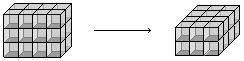
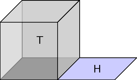
Products
Area = Length x Width
Volume = Length x Width x Height


\otimes
Univesality? Facing Torsion? Look down.
(v:K^a)\longrightarrow (u:K^b)\longrightarrow (vu^{\dagger} : \mathbb{M}_{a\times b}(K))
\otimes: K^a\times K^b\rightarrowtail \mathbb{M}_{a\times b}(K)
K^a\otimes K^b= \mathbb{M}_{a\times b}(K)
this defines matrices as a tensor product
\begin{matrix}
\otimes: & K^a & \to & K^b & \rightarrowtail & \mathbb{M}_{a\times b}(K)\\
& ~\downarrow X & & \downarrow Y & & \downarrow \widehat{X\otimes Y}\\
\langle t| :& U & \to & V & \rightarrowtail & W
\end{matrix}
Universal Mapping Property
\widehat{X\otimes Y}\left(\sum_i u_iv_i^{\dagger}\right) = \sum_i \langle t | Xu_i,Yv_i\rangle.
\mathbb{M}_{a\times b}(K)\oslash K^a\oslash K^b\to V_0\oslash K^a\oslash K^b
There is onto linear map:
V_2\otimes V_1 = \mathbb{M}_{d_2\times d_1}(K)/(R_2\otimes K^{d_1}+ K^{d_2}\otimes R_1)
Whitney products with torsion
0\to R_2 \to K^{d_2}\to V_2\to 0\\
0\to R_1 \to K^{d_1}\to V_1\to 0
\otimes
Quotient by an ideal to get exact sequence of tensors.

(Rows are exact sequences, columns are Curried bilinear maps.)
Tensor Ideals
*:U\times V\rightarrowtail W\\
X < U, Y < V, Z < W\\
\textnormal{ Submap if } X*Y \leq Z\\
\textnormal{ Left ideal if } U*Y \leq Z\\
\textnormal{ Right ideal if } X*V \leq Z
As with rings, ideals have quotients.
(A\otimes B)\otimes C \cong A\otimes (B\otimes C)\\
A\otimes B \cong B\otimes A\\
A\otimes K \cong A\\
(A\oslash B)\otimes_{\mathrm{End}(B)} B\cong A\\
(A\oslash B)\otimes (C\oslash D) \cong (A\otimes C)\oslash (B\otimes D)\\
(A\oslash B)\oslash (C\oslash D) \cong (A\oslash B)\otimes (D\oslash C)
A\oslash B\oslash C \cong \hom(C,\hom(B,A))\cong \hom(C\otimes B,A)\cong A\oslash (B\otimes C)
Fractional inspired notation for things known, e.g.:
(A\otimes B)\otimes C \cong A\otimes (B\otimes C)\\
A\otimes B \cong B\otimes A\\
A\otimes K \cong A\\
(A\oslash B)\otimes_{\mathrm{End}(B)} B\cong A\\
(A\oslash B)\otimes (C\oslash D) \to (A\otimes C)\oslash (B\otimes D)\\
(A\oslash B)\otimes (D\oslash C) \to (A\oslash B)\oslash (C\oslash D)
A\oslash B\oslash C \cong \hom(C,\hom(B,A))\cong \hom(C\otimes B,A)\cong A\oslash (B\otimes C)
Fractional inspired notation for things known, e.g.:
More accurately there are natural maps, invertible if f.d. over fields
Contractions


Add the values along the axis.
Perhaps weight by another tensor
then add.
Simplest example is the standard dot-product.
Uses? Averages, weighted averages, matrix multiplication, lets explore one called "convolution"...
Convolution
Goal: sharpen an image, find edges, find textures, etc.
In the past it was for "photo-shop" (is this trade marked?).
Today its image feature extraction to give to machine learning.
We turn the image into a (3 x 3 x ab)-tensor where very slice is a (3 x 3)-subimage.
Convolution with a target shape is a contraction on the (3 x 3)-face. Result is a ab-tensor (another (a x b)-image).
Do this with k-targets and get an (a x b x k) tensor with the meta-data of our image.
Machine Learner tries to learn these tensors.
                                                + + + + + + +
        * * * * *                             + + + + + + + + +
      * * * * * * *                         + + + +       + + + +
    * * * * * * * * *                       + + +           + + +
    * * * * * * * * *
    * * * * * * * * *
    * * * * * * * * *
    * * * * * * * * *                       - - -           - - -
      * * * * * * *                         - - - -       - - - -
        * * * * *                             - - - - - - - - -
                                                - - - - - - -
\begin{bmatrix}
a_{(i-1)(j-1)} & a_{(i-1)j} & a_{(i-1)(j+1)}\\
a_{i(j-1)} & a_{i(j+1)} & a_{i(j+2)}\\
a_{(i+1)(j-1)} & a_{(i+1)j} & a_{(i+1)(j+1)}\\
\end{bmatrix}
\bullet
\begin{bmatrix}
1 & 1 & 1\\
0 & 0 & 0\\
-1 & -1 & -1
\end{bmatrix}\qquad\qquad\\
\qquad=a_{(i-1)(j-1)}-a_{(i+1)(j-1)} + a_{(i-1)j}-a_{(i+1)j}+a_{(i-1)(j+1)}-a_{(i+1)(j+1)}
Some convolutions detect horizontal edges
                                                + +       - -
        * * * * *                             + + +       - - -
      * * * * * * *                         + + + +       - - - -
    * * * * * * * * *                       + + +           - - -
    * * * * * * * * *                       + +               - -
    * * * * * * * * *                       + +               - -
    * * * * * * * * *                       + +               - -
    * * * * * * * * *                       + + +           - - -
      * * * * * * *                         + + + +       - - - -
        * * * * *                             + + +       - - -
                                                + +       - -
\begin{bmatrix}
a_{(i-1)(j-1)} & a_{(i-1)j} & a_{(i-1)(j+1)}\\
a_{i(j-1)} & a_{i(j+1)} & a_{i(j+1)}\\
a_{(i+1)(j-1)} & a_{(i+1)j} & a_{(i+1)(j+1)}\\
\end{bmatrix}
\bullet
\begin{bmatrix}
-1 & 0 & 1\\
-1 & 0 & 1\\
-1 & 0 & 1
\end{bmatrix}\qquad\qquad\\
\qquad=-a_{(i-1)(j-1)}+a_{(i-1)(j+1)} - a_{i(j-1)}+a_{i(j+1)}-a_{(i+1)(j-1)}-a_{(i+1)(j+1)}
Some convolutions detect vertical edges
                                                  - - - - -
        * * * * *                               - + + + + + -
      * * * * * * *                           - +           + -
    * * * * * * * * *                       - +               + -
    * * * * * * * * *                       - +               + -
    * * * * * * * * *                       - +               + -
    * * * * * * * * *                       - +               + -
    * * * * * * * * *                       - +               + -
      * * * * * * *                           - +           + -
        * * * * *                               - + + + + + -
                                                  - - - - -
\begin{bmatrix}
a_{(i-1)(j-1)} & a_{(i-1)j} & a_{(i-1)(j+1)}\\
a_{i(j-1)} & a_{i(j+1)} & a_{i(j+1)}\\
a_{(i+1)(j-1)} & a_{(i+1)j} & a_{(i+1)(j+1)}\\
\end{bmatrix}
\bullet
\begin{bmatrix}
0 & -1 & 0\\
-1 & 4 & -1\\
0 & -1 & 0
\end{bmatrix}\qquad\qquad\\
\qquad=4a_{ij} - a_{(i-1)j}-a_{i(j-1)} + a_{i(j+1)}-a_{(i+1)j}
Some convolutions are good at all edges.

Most important contraction: generalized matrix multiplication

Further Flavors... including our logo :)


Operators
X = \begin{bmatrix} 1 & 1 & 1 \\ 1 & 1 & 1 \\ 1 & 1 & 0 \end{bmatrix}
t=\begin{bmatrix}1\\-1\\1\end{bmatrix}
t=\begin{bmatrix} 1\\ -1 \\ 1 \end{bmatrix} \to
Xt=\begin{bmatrix} 1\\ 1 \\ 0 \end{bmatrix} \to
X^2t=\begin{bmatrix} 2\\ 2 \\ 2 \end{bmatrix} \to
X^3 t=\begin{bmatrix} 4\\ 4 \\ 4 \end{bmatrix} \dashrightarrow
Stuff an infinite sequence
in a finite-dimensional space,
you get a dependence.
0=X^3t -2X^2 t=X^2(X-2I_3)t
So begins the story of annihilator polynomials and eigen values.
T =\begin{bmatrix} 1 & 0 & 3 \\ 4 & 5 & 6 \end{bmatrix}
X =\begin{bmatrix} 1 & 0 \\ 0 & 0 \end{bmatrix}
Y =\begin{bmatrix} 0 & 0 & 0 \\ 0 & 1 & 0 \\ 0 & 0 & 0
\end{bmatrix}.

(X^2-X)T\to x^2-x\\
T(Y^2-Y)\to y^2-y\\
XTY\to xy
An infinite lattice in finite-dimensional space makes even more dependencies.
(and the ideal these generate)
> M := Matrix(Rationals(), 2,3,[[1,0,2],[3,4,5]]);
> X := Matrix(Rationals(), 2,2,[[1,0],[0,0]] );
> Y := Matrix(Rationals(), 3,3,[[0,0,0],[0,1,0],[0,0,0]]);
> seq := [ < i, j, X^i * M * Y^j > : i in [0..2], j in [0..3]];
> U := Matrix( [s[3] : s in seq]);
        i   j   X^i * M * Y^j
        0   0   [ 1, 0, 2, 3, 4, 5 ]
        1   0   [ 1, 0, 2, 0, 0, 0 ]
        2   0   [ 1, 0, 2, 0, 0, 0 ]
        0   1   [ 0, 0, 0, 0, 4, 0 ]
        1   1   [ 0, 0, 0, 0, 0, 0 ]
        2   1   [ 0, 0, 0, 0, 0, 0 ]
        0   2   [ 0, 0, 0, 0, 4, 0 ]
        1   2   [ 0, 0, 0, 0, 0, 0 ]
        2   2   [ 0, 0, 0, 0, 0, 0 ]
        0   3   [ 0, 0, 0, 0, 4, 0 ]
        1   3   [ 0, 0, 0, 0, 0, 0 ]
        2   3   [ 0, 0, 0, 0, 0, 0 ]
In detail
Step out the bi-sequence
> E, T := EchelonForm( U );     // E = T*U
        0   0   [ 1, 0, 2, 3, 4, 5 ]    1
        1   0   [ 1, 0, 2, 0, 0, 0 ]    x
        0   1   [ 0, 0, 0, 0, 4, 0 ]    y
Choose pivots
Write null space rows as relations in pivots.
> A<x,y> := PolynomialRing( Rationals(), 2 );
> row2poly := func< k | &+[ T[k][1+i+3*j]*x^i*y^j :
     i in [0..2], j in [0..3] ] );
> polys := [ row2poly(k) : k in [(Rank(E)+1)..Nrows(E)] ];
        2   0   [ 1, 0, 2, 0, 0, 0 ]    x^2 - x
        1   1   [ 0, 0, 0, 0, 0, 0 ]    x*y
        2   1   [ 0, 0, 0, 0, 0, 0 ]    x^2*y
        0   2   [ 0, 0, 0, 0, 4, 0 ]    y^2 - y
        1   2   [ 0, 0, 0, 0, 0, 0 ]    x*y^2
        2   2   [ 0, 0, 0, 0, 0, 0 ]    x^2*y^2
        0   3   [ 0, 0, 0, 0, 4, 0 ]    y^3 - y
        1   3   [ 0, 0, 0, 0, 0, 0 ]    x*y^3
        2   3   [ 0, 0, 0, 0, 0, 0 ]    x^2*y^3
> ann := ideal< A | polys >;
> GroebnerBasis(ann);
    x^2 - x,
    x*y,
    y^2 - y
Take Groebner basis of relation polynomials
Groebner in bounded number of variables is in polynomial time (Bradt-Faugere-Salvy).
T =\begin{bmatrix} 1 & 0 & 3 \\ 4 & 5 & 6 \end{bmatrix}
I_2- X =\begin{bmatrix} 0 & 0 \\ 0 & 1 \end{bmatrix}
I_3- Y =\begin{bmatrix} 1 & 0 & 0 \\ 0 & 0 & 0 \\ 0 & 0 & 1
\end{bmatrix}.
(X^2-X)T\to x^2-x\\
T(Y^2-Y)\to y^2-y

Same tensor,
different operators,
can be different annihilators.
T =\begin{bmatrix} 1 & 2 & 3 \\ 4 & 5 & 6 \end{bmatrix}
X =\begin{bmatrix} 1 & 0 \\ 0 & 0 \end{bmatrix}
Y =\begin{bmatrix} 0 & 0 & 0 \\ 0 & 1 & 0 \\ 0 & 0 & 0
\end{bmatrix}.
(X^2-X)T\to x^2-x\\
T(Y^2-Y)\to y^2-y
Different tensor,
same operators,
can be different annihilators.

Data
T:\mathbb{M}_{a\times b}(K), X:\mathbb{M}_a(K), Y:\mathbb{M}_b(K)
Action by polynomials
a(x,y)\cdot T
= \left(\sum_{i,j:\mathbb{N}} \alpha_{ij} x^i y^j\right)\cdot T
= \sum_{i,j:\mathbb{N}}\alpha_{ij} X^iT Y^j.
Resulting annihilating ideal
\mathrm{ann}_{X,Y}(T) = \{
a(x,y):K[x,y]\mid
a(X,Y)T=0\}.
Could this be wild? Read below.
Annihilators
Mal'cev showed that the representation of 2-generated algebras is "wild" in that its theory is undecidable.
However, we have two features: our variables commute, and our operators are transverse.
Still, maybe this is wild?
Transverse Operators
\mathbb{M}_{ab}(K) \cong \mathbb{M}_a(\mathbb{M}_b(K))
\cong \mathbb{M}_a(K)\otimes \mathbb{M}_b(K)
\mathbb{M}_a(K)\times \mathbb{M}_b(K)\rightarrowtail \mathbb{M}_{ab}(K)
This presecirbes a bimap
The image of this map we call the transverse operators.
These generate all other operators.
Explore a proof below or move on to more generality


(\rho:K[x_0,\ldots,x_{\ell}]\to \mathrm{End}(V_0\oslash\cdots\oslash V_{\ell}))
(\omega:\prod_a \mathrm{End}(V_a))\to
Claim
Kernel is the annihilator of the operator.
Theorem. A Groebner basis for this annihilator can be computed in polynomial time.
(\omega:\mathrm{End}(V)) \longrightarrow (\rho:K[x]\to \mathrm{End}(V))
Fact.
(\omega:\prod_{a=0}^{\ell} \mathrm{End}(V_a)) \longrightarrow
\mathrm{End}(V_0\oslash\cdots \oslash V_{\ell})\cong \frac{V_0\oslash\cdots\oslash V_{\ell}}{V_0\oslash\cdots\oslash V_{\ell}}
\cong \frac{(V_0\oslash\cdots \oslash V_{\ell-1})}{(V_0\oslash\cdots \oslash V_{\ell-1})}\otimes \frac{V_{\ell}}{V_{\ell}}
\qquad \vdots\\
\qquad \cong (V_0\oslash V_0)\otimes \cdots\otimes (V_{\ell}\oslash V_{\ell})\\
\qquad = \mathrm{End}(V_0)\otimes\cdots\otimes \mathrm{End}(V_{\ell})
\mathrm{End}(V) = V\oslash V = \frac{V}{V}
\frac{A\oslash B}{C\oslash D} \cong \frac{A}{B}\otimes \frac{D}{C}
Annihilators General
\mathrm{ann}_{\omega}(t) = \{ a(X):K[X]\mid \langle t|a(X) =0 \}
a(X)=\sum_{e:[\ell]\to \mathbb{N}} \alpha_e X^e\longrightarrow \\
\qquad 0=\sum_{e} \alpha_e \omega_0^{e_0} \langle t | \omega_{\ell}^{e_{\ell}}v_{\ell},\ldots,\omega_1^{e_1} v_1\rangle


Open
- Find more examples of matrices whose traits are parabolic (known), hyperbolic (known), elliptic (not known).
- Find a family of matrices with a trait that has genus, can all ellipitic curves appear?
- Is every ideal possible as an annihilator?
Traits
Prime & Primary Factors
- Unique by Lasker-Noether (below)
- Computable by Groebner basis
- Generalize eigen theory of operators on a single vector space.
- Problem: primes almost always determined by axis, often 0-dimensional, i.e. just eigen values.
A trait is an element of the Groebner basis of a prime decomposition of the annihilator.
Traits generalize eigen values.
In K[x]
Lasker-Noether: In K[X]
I = (a_1(x)^{e_1})\cap\cdots \cap (a_{m}(x)^{e_m})
a_i(x) \textnormal{ no proper factors}
I=Q_1\cap\cdots \cap Q_m
\sqrt{Q_i}=\{ a(X):K[X]\mid (\exists e:\mathbb{N})(a(X)^e:Q_i)\}
are all prime, and the minimal primes are unique.
where
\sqrt{(x^2-x,y^2-y,xy)} = (x,y) = \sqrt{(x^2-x,y^2-y)}
As a variety we only see the radical, i.e. that x=0 and y=0.
There is nothing about the tensor in this.
Need to look at the scheme -- need to focus on the xy.
Isolating Traits
Z(S,P) = \{ \omega:\prod_{a:[\ell]} \mathrm{End}(V_a) \mid \langle S| P(\omega) = 0\}
(S<:T)\longrightarrow (P<: K[X])\longrightarrow
Examples
\langle t | u,v\rangle = u^{\dagger}Jv,\qquad J=\begin{bmatrix} 0 & I_m\\ -I_m & 0 \end{bmatrix}
P=(x_2x_1-1)
Z(t,P) = \{ (F_2,F_1)\mid F_2^{\dagger}JF_1 = J \} = \mathrm{Sim}(J)\\
\qquad = \mathrm{Sp}(2m,K)K^{\times}
Ideals for operator sets
I(S,\Delta) = \{ p(X):K[X] \mid \langle S| p(\Delta) = 0\}
(S<:T)\longrightarrow (\Delta<: \prod_{a:[\ell]} \mathrm{End}(V_a))\longrightarrow
This ideal is the intersection of annihilators for each operator. So the dimension of the ideal grows.
This is how we isolate traits of high dimension -- use many operators.
Tensors with traits
T(P,\Delta) = \{ t:T \mid \langle t| P(\Delta) = 0\}
(S<:T)\longrightarrow (\Delta<: \prod_{a:[\ell]} \mathrm{End}(V_a))\longrightarrow
T-sets are to traits what eigen vectors are to eigen values.

The Correspondence Theorem (First-Maglione-W.)
This is a ternary Galois connection.
Summary of Trait Theorems (First-Maglione-W.)
- Linear traits correspond to derivations.
- Monomial traits correspond to singularities
- Binomial traits are only way to support groups.
For trinomial ideals, all geometries can arise so classification beyond this point is essentially impossible.
Derivations & Densors
Most influential Traits
Idea: study the hypersurface traits -- captures the largest swath of operators. Reciprocally, what we find applies to very few tensors, perhaps even just the one we study.
Fact: In projective geometry there is a well-defined notation of a generic degree d hyper surface:
g_1(x_0,\ldots,x_{\ell}) = \sum_{a=0}^{\infty} \alpha_a x_a\qquad \qquad\qquad \alpha_a\neq 0\\
g_2(x_0,\ldots,x_{\ell}) = \sum_{a=0}^{\ell}\sum_{b=a}^{\ell} \alpha_{ab} x_a x_b,\qquad \alpha_{ab}\neq 0\\
\cdots
Seems tractible only for the linear case
Derivations & Densors
Treating 0 as contra-variant the natural hyperplane is:
D(x_0,\ldots,x_{\ell}) = -x_0 + x_1+\cdots + x_{\ell}
That is, the generic linear trait is simply to say that operators are derivations!
\langle t | D(\delta) |v\rangle=0 \equiv\\
\delta_0 \langle t|v\rangle = \langle t|\delta_{\ell} v_{\ell},\cdots ,v_1\rangle+\cdots+\langle t|v_{\ell},\ldots,\delta_1 v_1\rangle
However, the schemes Z(S,P) are not the same as Z(P), so generic here is not the same as generic there...work required.
Derivations are Universal Linear Operators
Theorem (FMW). If
2.~ P=(\sum_{a} \alpha_{1a} x_a, \cdots, \sum_a \alpha_{ma} x_a)
Then
3.~(\forall a:[\ell])(\exists i:[m])(\alpha_{ia}\neq 0)
1. |K|>\ell
(\exists \omega:\prod_{a=0}^{\ell} K^{\times}) ( Z(S,P)^{\omega} <: \mathrm{Der}(S) )
(If 1. fails extend the field; if 2. is affine, shift; if 3 fails, then result holds over support of P.)
Unintended Consequences
Since Whitney's 1938 paper, tensors have been grounded in associative algebras.
(A<: \mathrm{End}(U)^{op}\times \mathrm{End}(V))\to U\otimes_A V
Derivations form natural Lie algebras.
[\delta,\delta'] = ([\delta'_0,\delta_0] , [\delta_1,\delta'_1],\ldots,[\delta_{\ell},\delta'_{\ell}] )\qquad\qquad\qquad \\
\qquad =(\delta'_0\delta_0-\delta_0\delta'_0,\delta_1\delta'_1-\delta'_1\delta_1,\ldots,\delta_{\ell}\delta'_{\ell}-\delta'_{\ell}\delta_{\ell})
If associative operators define tensor products but Lie operators are universal, who is right?
Tensor products are naturally over Lie algebras
Theorem (FMW). If
(\omega,\omega':Z(S,P)) \to\hspace{5cm}\\
\qquad(\omega_a\bullet \omega'_a = \alpha_{a}\omega_a\omega'_a+\beta_a \omega'_a\omega_a : Z(S,P))
Then in all but at most 2 values of a
\langle (\alpha_a,\beta_a)\rangle = \langle (1,-1)\rangle \textnormal{ i.e. a Lie bracket}
In particular, to be an associative algebra we are limited to at most 2 coordinates. Whitney's definition is a fluke.
Module Sides no longer matter
- Whitney tensor product pairs a right with a left module, often forces technical op-ring actions.
- Lie algebras are skew commutative so modules are both left and right, no unnatural op-rings required.
V_1\otimes_{A_{10}} V_0 \textnormal{ vs. } V_0\otimes_{??} V_1
Associative Laws no longer
- Whitney tensor product is binary, so combining many modules consistantly by associativity laws isn't always possible - different coefficient rings.
(V_3\otimes_{A_{32}} V_2)\otimes_{A_{(32)1}} V_1 \textnormal{ vs. }
V_3\otimes_{??} (V_2\otimes_{??} V_1)
- Lie tensor products can be defined on arbitrary number of modules - no need for associative laws.
(\Delta<: \prod_{a:[\ell]} \mathfrak{gl}(V_a)) \to \hspace{2cm}\\
\qquad (| V_{\ell},\ldots,V_0 |)_{\Delta}=T(\Delta,D)
Missing opperators
- Whitney tensor product puts coefficient between modules only, cannot operate at a distance.
As valence grows we act on a linear number of spaces but have exponentially many possible actions left out.
V_3\otimes_{A_{32}} V_2\otimes_{A_{21}} V_1\textnormal{ vs. }
V_3\otimes_{A_{31}} V_1\otimes_{A_{12}} V_2
Lie tensor products act on all sides.
Densor
(\Delta<: \prod_{a:[\ell]} \mathfrak{gl}(V_a)) \to \hspace{2cm}\\
\qquad (| V_{\ell},\ldots,V_0 |)_{\Delta}=T(\Delta,D)
Densors are
- agnostic to sides of modules -- no comm. laws.
- n-ary needing no associative laws.
- operators are on all sides
- ...and Whitney products are actually just a special case of densors.
Monomials, Singularities, & simplicial complexes
(\langle t|U_A, V_{\bar{A}}\rangle =0)\quad \leftrightarrow \quad (X^e: I(t, \Omega_A), e=\chi_A)
Local Operators
(A <: [\ell]) \to ((a:A)\to (U_a<:V_a))\longrightarrow\\
\qquad\Omega_A =\prod_{a:A} U_a\oslash V_a\times \prod_{a:\bar{A}} V_a\oslash V_a
I.e. operators that on the indices A are restricted to the U's.
Claim. Singularity at U if, and only if, monomial trait on A.
Singularities come with traits that are in bijection with Stanley-Raisner rings, and so with simplicial complexes.

Shaded regions are 0.
Binomials & Groups
Theorem (FMW). If for every S and P
(\omega,\omega'\in Z(S,P))\to (a:[\ell])\to
((\omega_a\omega'_a)^{\pm 1}=:Z(S,P))
P=(X^{e_1}-X^{f_1},\ldots, X^{e_m}-X^{f_m})
(i,j:[1..m])\to (a:[\ell]) \to (e_i(a)+f_j(a)\leq 1)
then
If
then the converse holds.
(We speculate this is if, and only if.)
Implication
- Classifies the categories of tensors with transverse operators (there are as many as the valence).
Under symmetry...
P<:K[x_0,x_1,x_2; \sigma=(1,2)]
Z(S,P)^{\sigma} = \{ \omega:Z(S,P)\mid (a:[\ell])\to \omega_{a\sigma}=\omega_a) \}
Z(S,x_2x_1-1)^{(1,2)} = \mathrm{Isom}(S).
In many settings a symmetry is required. The correspondence applies here but the classifications just given all evolve. Much to be learned here. E.g.
Application: Decompositions
Tensor & Their Operators
By James Wilson
Tensor & Their Operators
Definitions and properties of tensors, tensor spaces, and their operators.


