Equiangular Tight Frames

John Jasper
South Dakota State University
MRI: Resolution v. Scan Time

Pixels
Time

High resolution \(\Longleftrightarrow\) Long scan time
Real world signals are sparse.
\(\Downarrow\)
The conventional tradeoff is a lie!
We can solve "underdetermined"
\[Ax=b\] by \(L^{1}\) minimization provided:
- \(x\) is sparse, and
- Columns of \(A\) are "spread out"
Pixels
Time

Compressed Sensing

We need an image with many pixels:


\(=\)
Image

Transformed Image


- A measurement is a single dot product
- Using old linear algebra we need as many dot products as pixels
- Under an invertible transformation the image is sparse (lots of zeros)
Compressed Sensing

We need an image with many pixels:

\(=\)

Transformed Image

Column vectors need to be "spread out" in space
- For sparse signals we need a lot fewer measurements
- But the columns of our sensing matrix must be "spread out" in space
Roadmap for this talk

Compressed Sensing
Vectors that are "Spread out"
Equiangular tight frames
ETFs from groups
\(\Z_{2}\times\Z_{2}\times\Z_{2}\times\Z_{2}\)
The design theory underneath

Real Flat ETFs

Some binary codes
Group divisible designs
ETFs and graphs

Definition. Given unit vectors \(\Phi=(\varphi_{i})_{i=1}^{N}\), we define the coherence
\[\mu(\Phi) = \max_{i\neq j}|\langle \varphi_{i},\varphi_{j}\rangle|.\]
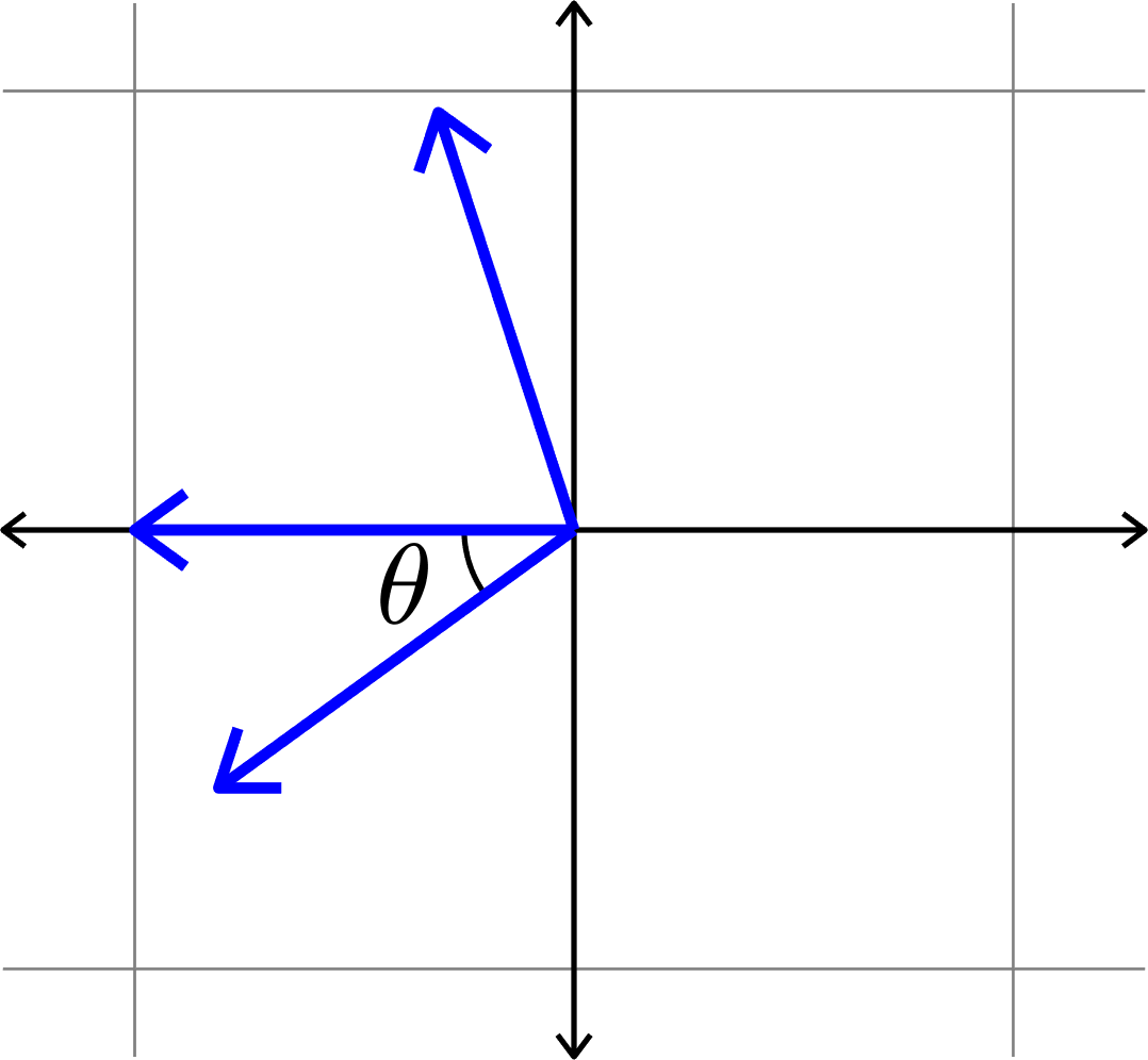
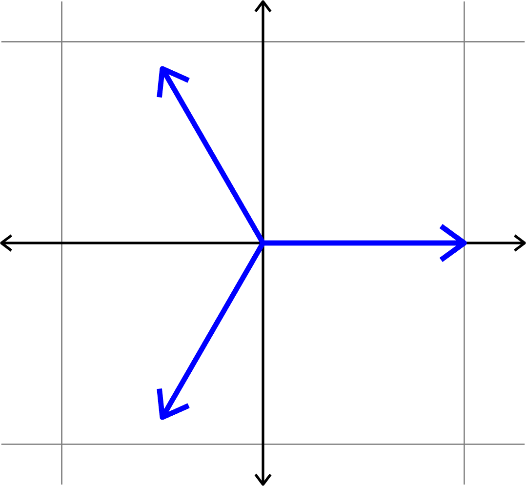
Measuring how "spread out" vectors are
\[\mu(\Phi) = \cos(\theta)\]

\(\mu(\Phi) = \cos(\theta)\)??
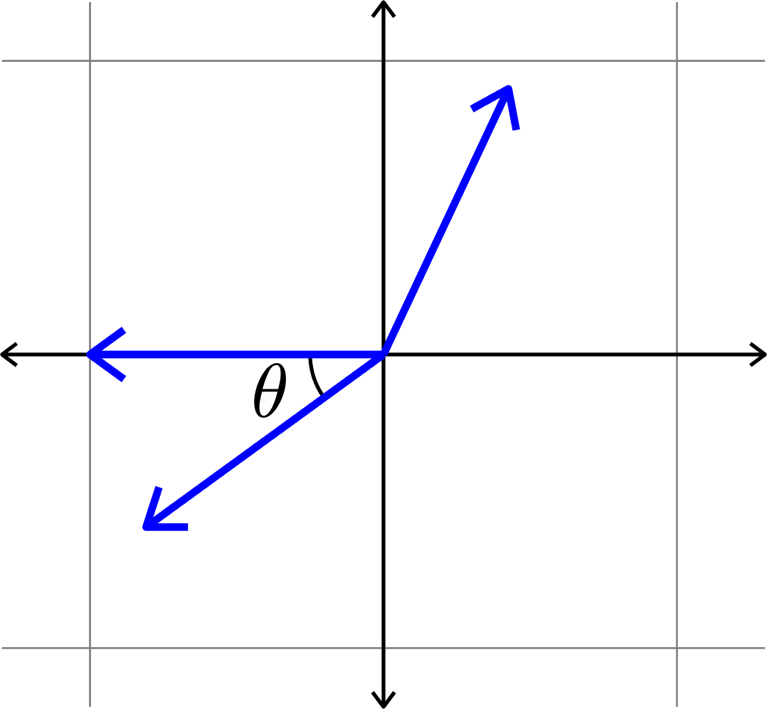

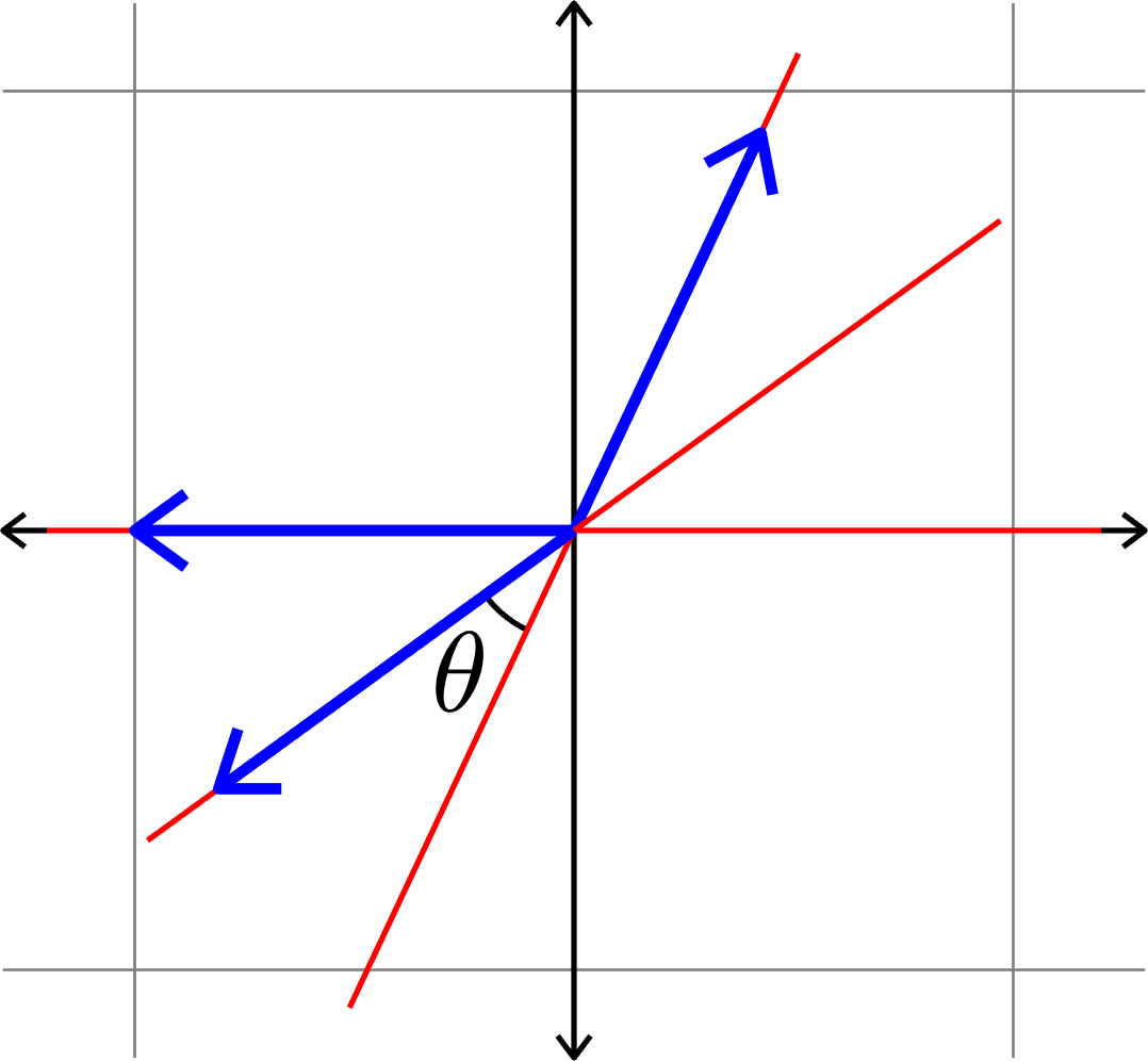
\(\mu(\Phi) = \cos(\theta)\)
Measuring how "spread out" vectors are
Definition. Given unit vectors \(\Phi=(\varphi_{i})_{i=1}^{N}\), we define the coherence
\[\mu(\Phi) = \max_{i\neq j}|\langle \varphi_{i},\varphi_{j}\rangle|.\]

Example.
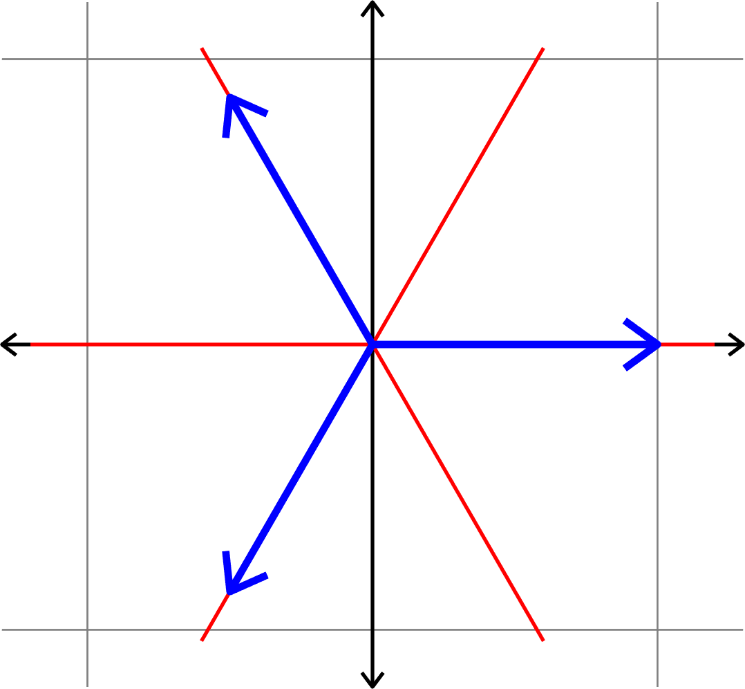
Measuring how "spread out" vectors are
Definition. Given unit vectors \(\Phi=(\varphi_{i})_{i=1}^{N}\), we define the coherence
\[\mu(\Phi) = \max_{i\neq j}|\langle \varphi_{i},\varphi_{j}\rangle|.\]
Vectors that are as spread out as possible
Theorem (the Welch bound). Given a collection of unit vectors
\(\Phi=(\varphi_{i})_{i=1}^{N}\) in \(\mathbb{C}^d\), the coherence satisfies
\[\mu(\Phi)\geq \sqrt{\frac{N-d}{d(N-1)}}.\]
Equality holds if and only if the following two conditions hold:
- Tight: There is a constant \(A>0\) such that \[\sum_{i=1}^{N}|\langle v,\varphi_{i}\rangle|^{2} = A\|v\|^{2} \quad\text{for all } v.\]
- Equiangular: There is a constant \(\alpha\) such that \[|\langle\varphi_{i},\varphi_{j}\rangle| = \alpha\quad\text{for all }i\neq j.\]
Welch bound equality \(\Longleftrightarrow\) equiangular tight frame (ETF)
Tightness and short, fat matrices
Useful matrix representation: \(\quad\Phi = \begin{bmatrix} | & | & & |\\ \varphi_{1} & \varphi_{2} & \cdots & \varphi_{N}\\ | & | & & |\end{bmatrix}\)
Tightness: There is a constant \(A>0\) such that \[\sum_{i=1}^{N}|\langle v,\varphi_{i}\rangle|^{2} = A\|v\|^{2} \quad\text{for all } v.\]

( )
\(\Leftrightarrow\quad\Phi\Phi^{\ast} = AI\)
\(\Leftrightarrow\quad\) the rows of \(\Phi\) are orthogonal and equal norm
\(\langle v,\Phi\Phi^{\ast}v\rangle = \)
\(\langle v,\Phi\Phi^{\ast}v\rangle = \)
Examples of equiangular tight frames
Example 2. Consider the (multiple of a) unitary matrix

Example 1. Consider the (multiple of a) unitary matrix
\[\left[\begin{array}{rrrr}1 & -1 & 1 & -1\\ 1 & 1 & -1 & -1\\ 1 & -1 & -1 & 1\end{array}\right]\]
\[\left[\begin{array}{rrrr} 1 & 1 & 1 & 1\\ 1 & -1 & 1 & -1\\ 1 & 1 & -1 & -1\\ 1 & -1 & -1 & 1\end{array}\right]\]
\[\left[\begin{array}{rrrr} 1 & 1 & 1\\ \sqrt{2} & -\sqrt{\frac{1}{2}} & -\sqrt{\frac{1}{2}}\\ 0 & \sqrt{\frac{3}{2}} & -\sqrt{\frac{3}{2}}\end{array}\right]\]
\[\left[\begin{array}{rrrr}\sqrt{2} & -\sqrt{\frac{1}{2}} & -\sqrt{\frac{1}{2}}\\ 0 & \sqrt{\frac{3}{2}} & -\sqrt{\frac{3}{2}}\end{array}\right]\]

Examples of equiangular tight frames
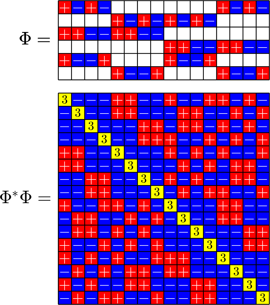
Example 3.


Theme of the talk:

\(\mathbb{Z}_{2}\times\mathbb{Z}_{2}\times\mathbb{Z}_{2}\times\mathbb{Z}_{2}\)

Some ETFs
arise from
groups...
a lot more ETFs
arise from
combinatorial designs!
M
Roadmap for this talk

Compressed Sensing

Vectors that are "Spread out"

Equiangular tight frames
ETFs from groups
\(\Z_{2}\times\Z_{2}\times\Z_{2}\times\Z_{2}\)
The design theory underneath

Real Flat ETFs

Some binary codes
Group divisible designs
ETFs and graphs

\[\Z_{7}\left\{\begin{array}{c} 0\\ 1\\ 2\\ 3\\ 4\\ 5\\ 6 \end{array}\right. \left[\begin{array}{ccccccc} 1 & 1 & 1 & 1 & 1 & 1 & 1\\ 1 & \omega & \omega^2 & \omega^3 & \omega^4 & \omega^5 & \omega^6\\ 1 & \omega^2 & \omega^4 & \omega^6 & \omega & \omega^3 & \omega^5\\ 1 & \omega^3 & \omega^6 & \omega^2 & \omega^5 & \omega & \omega^4\\ 1 & \omega^4 & \omega & \omega^5 & \omega^2 & \omega^6 & \omega^3\\ 1 & \omega^5 & \omega^3 & \omega & \omega^6 & \omega^4 & \omega^2\\ 1 & \omega^6 & \omega^5 & \omega^4 & \omega^3 & \omega^2 & \omega \end{array}\right]\]
\[\begin{array}{c} 1\\ 2\\ 4 \end{array}\left[\begin{array}{ccccccc} 1 & \omega & \omega^2 & \omega^3 & \omega^4 & \omega^5 & \omega^6\\ 1 & \omega^2 & \omega^4 & \omega^6 & \omega & \omega^3 & \omega^5\\ 1 & \omega^4 & \omega & \omega^5 & \omega^2 & \omega^6 & \omega^3 \end{array}\right]\]
Rows from a DFT
(\(\omega = e^{2\pi i/7}\))
\[\Phi = \left[\begin{array}{ccccccc} 1 & \omega & \omega^2 & \omega^3 & \omega^4 & \omega^5 & \omega^6\\ 1 & \omega^2 & \omega^4 & \omega^6 & \omega & \omega^3 & \omega^5\\ 1 & \omega^4 & \omega & \omega^5 & \omega^2 & \omega^6 & \omega^3 \end{array}\right]\]
Rows from a DFT
\(\Phi\) is tight, since it is rows out of a unitary.
\(\Phi\) is equiangular, since \(D=\{1,2,4\}\subset\Z_{7}\) is a difference set.
That is, if we look at the difference table
\[\begin{array}{r|rrr} - & 1 & 2 & 4\\ \hline 1 & 0 & 6 & 4\\ 2 & 1 & 0 & 5\\ 4 & 3 & 2 & 0 \end{array}\]
every nonidentity group element shows up the same number of times
Difference sets \(\Rightarrow\) equiangular?
\(\Phi^{\ast}\Phi = \operatorname{circ}(\hat{\mathbf{1}}_{D})\)
\(|\Phi^{\ast}\Phi|^{2} = \operatorname{circ}\big(|\hat{\mathbf{1}}_{D}|^{2}\big)\)
\(|\hat{\mathbf{1}}_{D}|^{2} = \hat{\mathbf{1}}_{D}\odot\overline{\hat{\mathbf{1}}_{D}} = \mathcal{F}\big(\mathbf{1}_{D}\ast \mathbf{1}_{-D}\big) \)
Want \(\Phi=\) ETF, i.e., \(|\hat{\mathbf{1}}_{D}|^{2} = a\delta_{0}+b\mathbf{1}_{G} = \textit{spike + flat}\)
\(\mathcal{F}(\textit{spike + flat}) = \textit{spike + flat}\)
\(\mathbf{1}_{D}\ast \mathbf{1}_{-D}=\textit{spike + flat}\quad\Longleftrightarrow\quad D\) is a difference set
Suppose: \(\Phi=(\text{rows of DFT indexed by }D)\)
Meme of the talk:

\(\mathbb{Z}_{2}\times\mathbb{Z}_{2}\times\mathbb{Z}_{2}\times\mathbb{Z}_{2}\)

Some ETFs
arise from
McFarland Difference Sets...
a lot more ETFs
arise from
Steiner systems!
\[\begin{array}{c|cccccc} & (0,0,0,1) & (1,1,0,1) & (0,0,1,0) & (1,0,1,0) & (0,0,1,1) & (0,1,1,1)\\ \hline (0,0,0,1) & (0,0,0,0) & (1,1,0,0) & (0,0,1,1) & (1,0,1,1) & (0,0,1,0) & (0,1,1,0)\\ (1,1,0,1) & (1,1,0,0) & (0,0,0,0) & (1,1,1,1) & (0,1,1,1) & (1,1,1,0) & (1,0,1,0)\\ (0,0,1,0) & (0,0,1,1) & (1,1,1,1) & (0,0,0,0) & (1,0,0,0) & (0,0,0,1) & (0,1,0,1)\\ (1,0,1,0) & (1,0,1,1) & (0,1,1,1) & (1,0,0,0) & (0,0,0,0) & (1,0,0,1) &(1,1,0,1)\\ (0,0,1,1) & (0,0,1,0) & (1,1,1,0) & (0,0,0,1) & (1,0,0,1) & (0,0,0,0) & (0,1,0,0)\\ (0,1,1,1,) & (0,1,1,0) & (1,0,1,0) & (0,1,0,1) & (1,1,0,1) & (0,1,0,0) & (0,0,0,0) \end{array}\]
\[D=\{(0,0,0,1),(0,0,1,0),(0,0,1,1),(0,1,1,1),(1,0,1,0),(1,1,0,1)\}\]
is a (McFarland) difference set in \(G=\Z_{2}\times\Z_{2}\times\Z_{2}\times\Z_{2}\)
A McFarland difference set
The subgroup \[H=\Z_{2}\times \Z_{2}\times 0\times 0\leqslant G\] is disjoint from \(D\).
A McFarland difference set
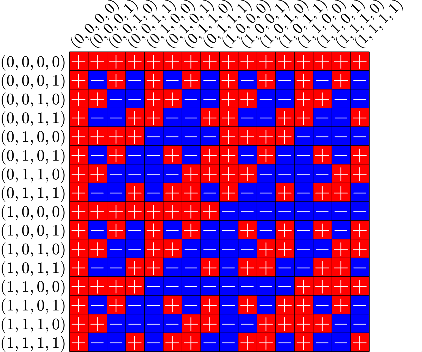
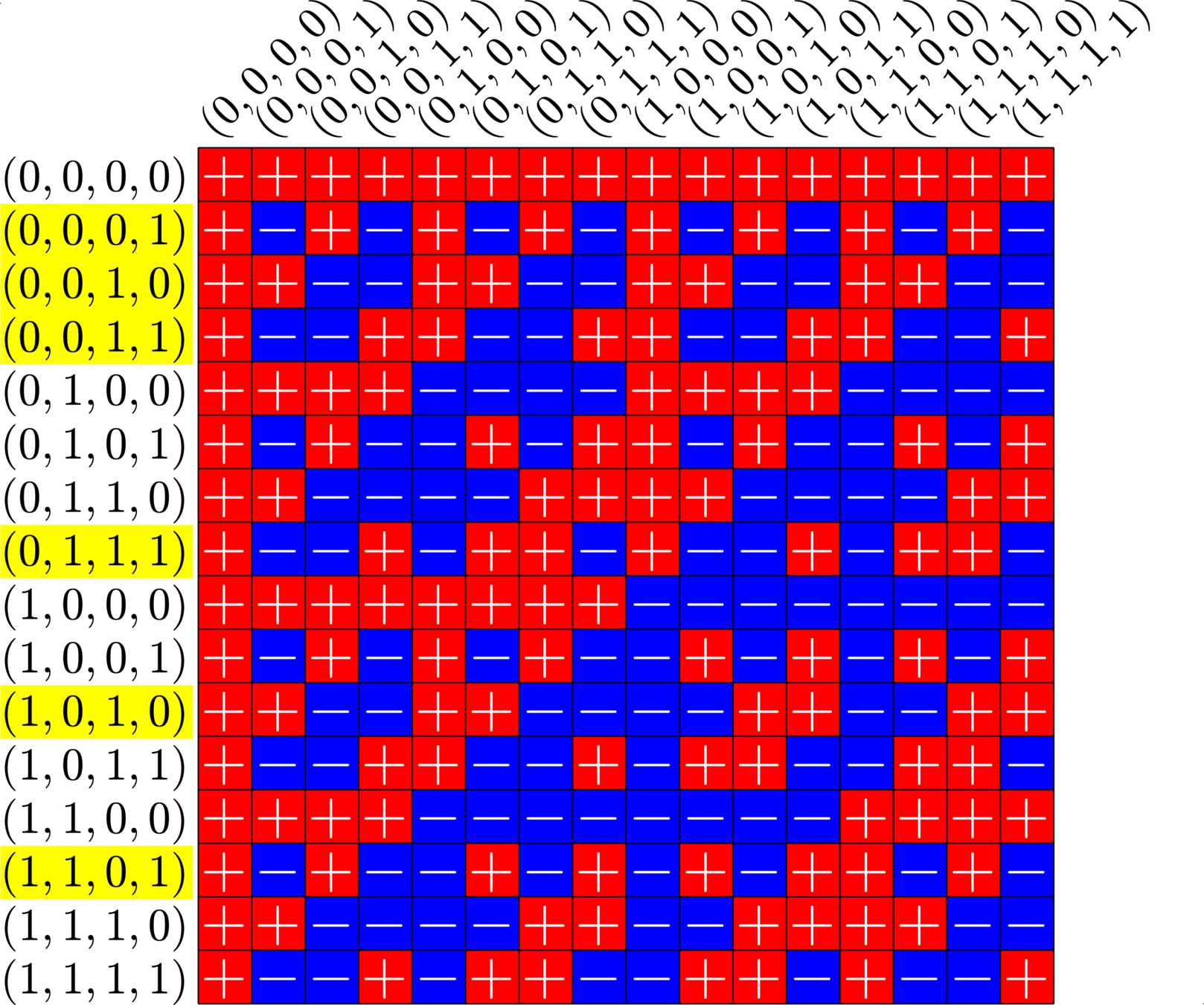
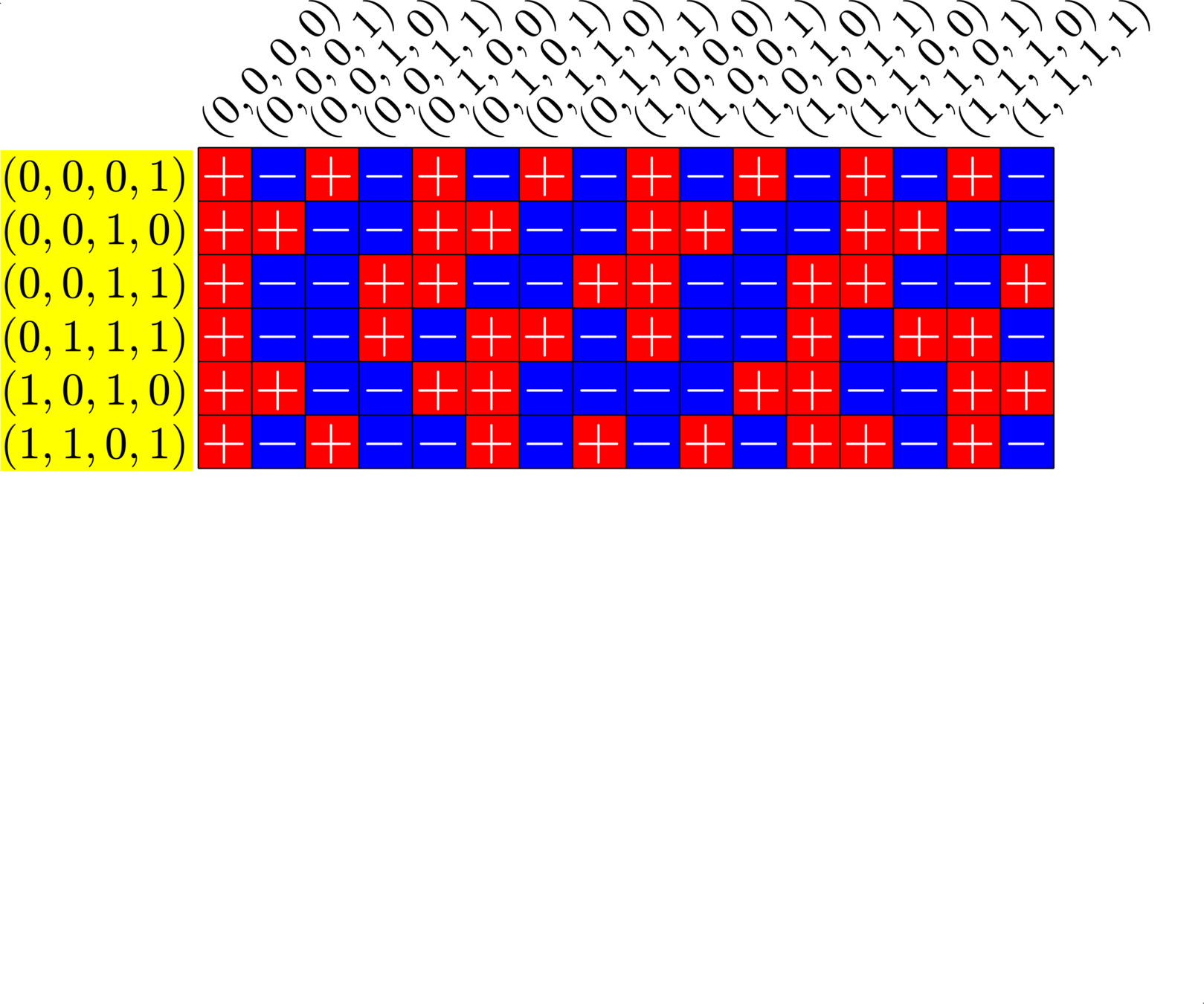
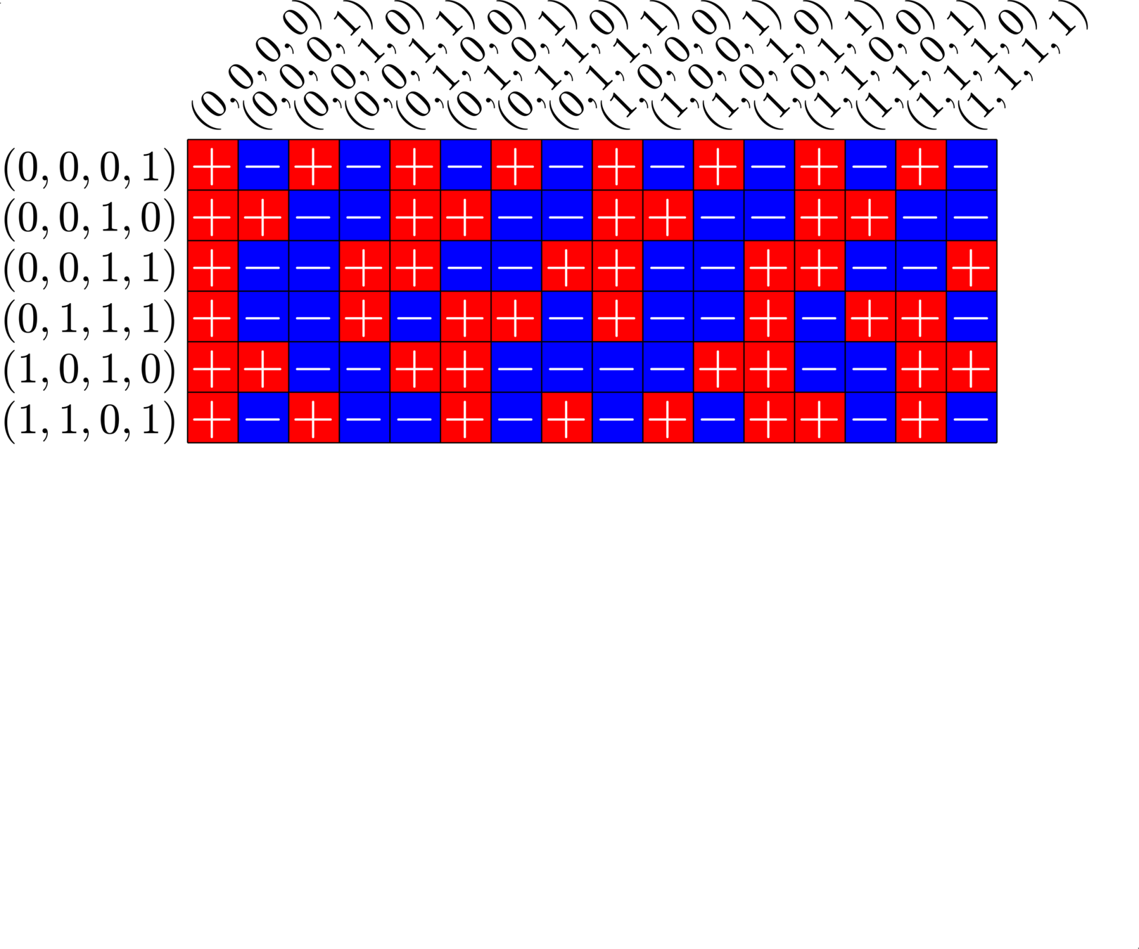
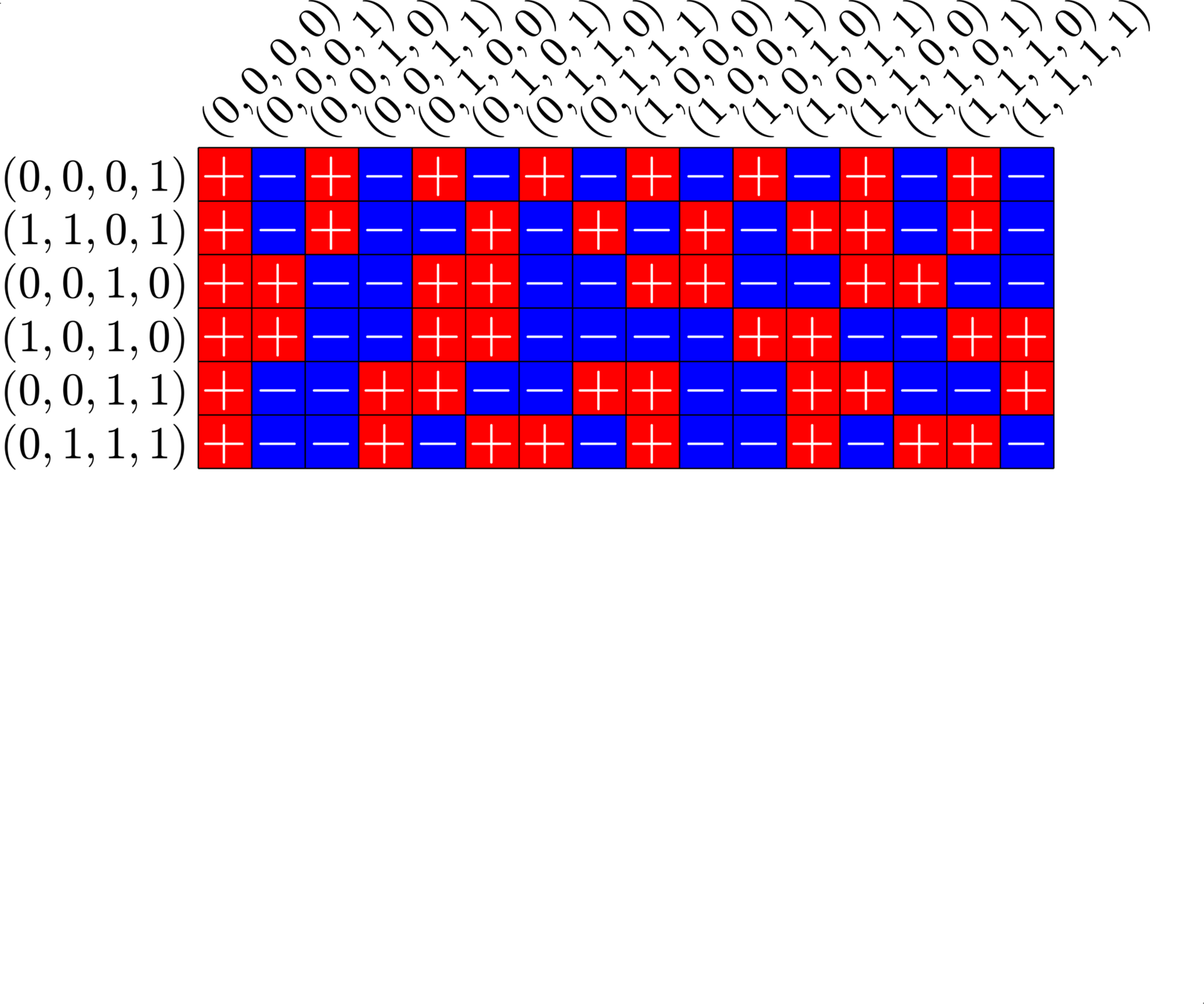

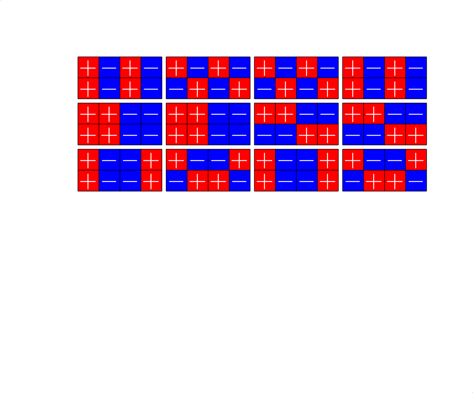
Steiner Systems
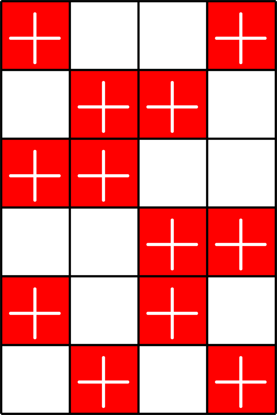
Definition. A \((2,k,v)\)-Steiner system is a \(\{0,1\}\)-matrix \(X\) such that:
- Each row of \(X\) has exactly \(k\) ones.
- Each column of \(X\) has exactly \(r=\frac{v-1}{k-1}\) ones.
- The dot product of any pair of distinct columns is one.
Example. The matrix
\(X = \)
is a \((2,2,4)\)-Steiner system.

The Star Product
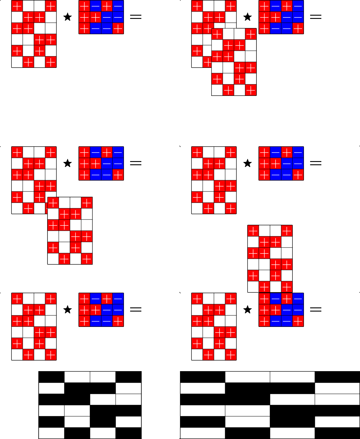
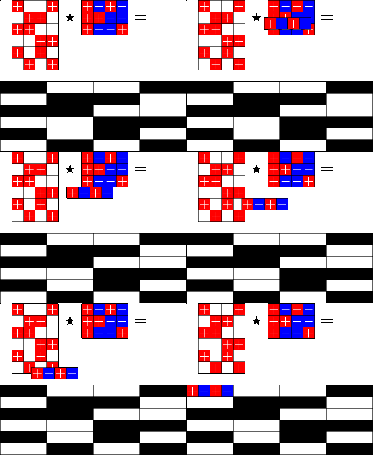
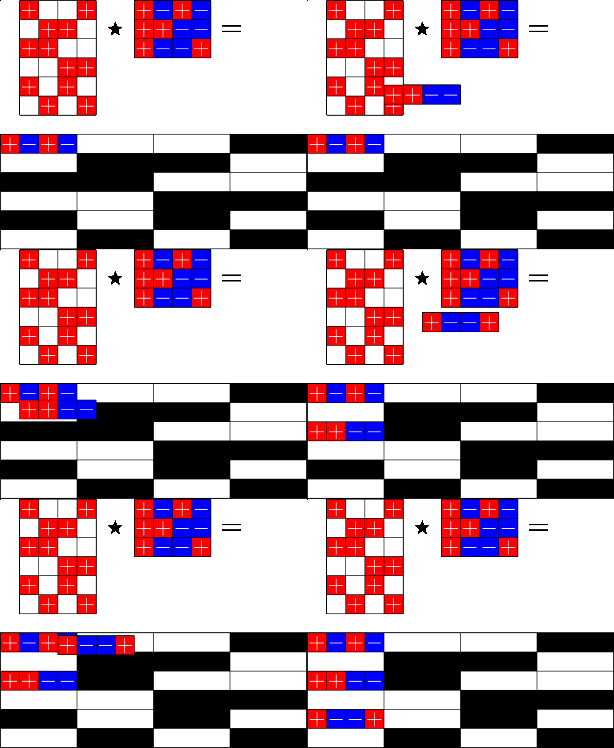
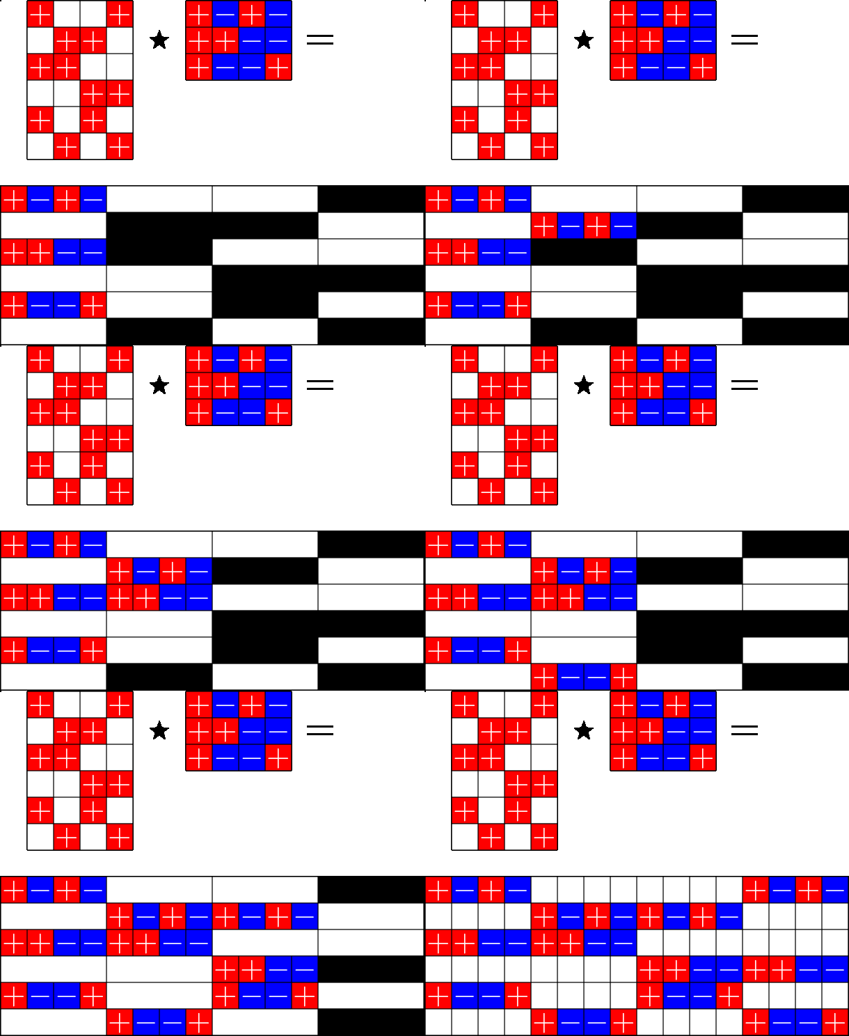
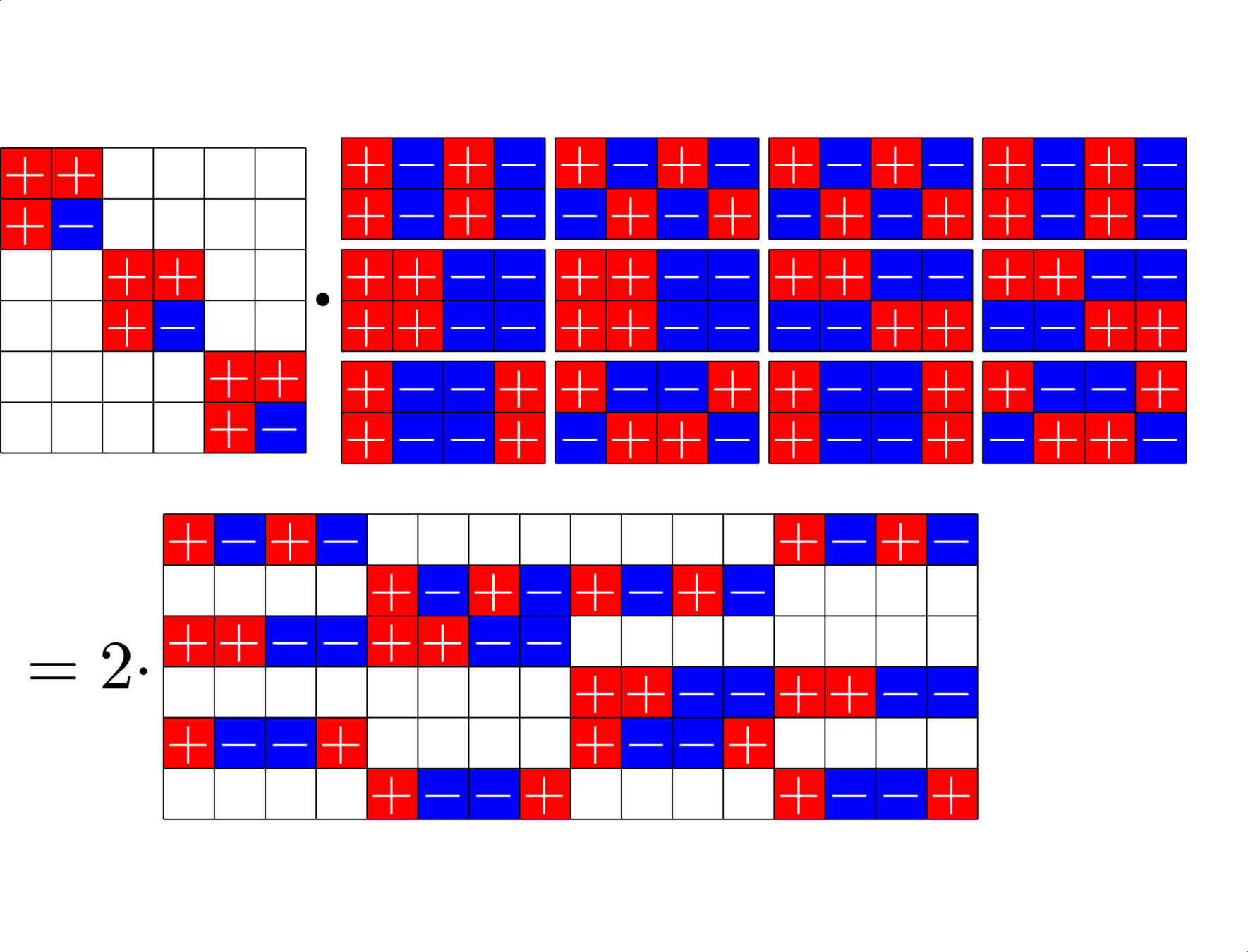
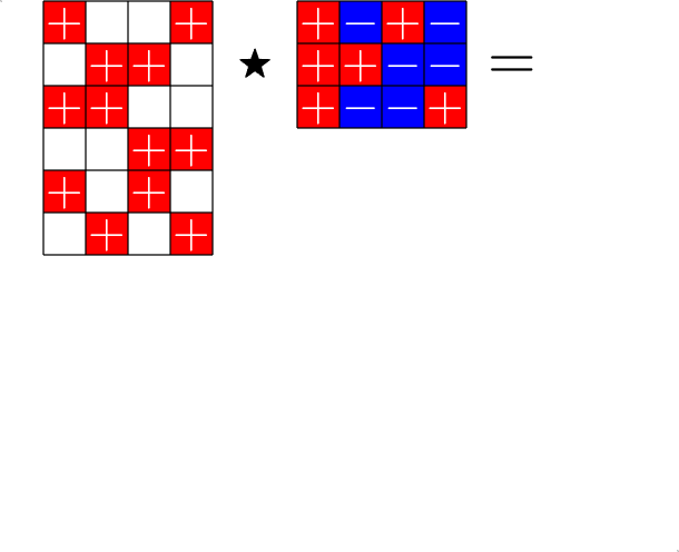
A way to construct lots of ETFs

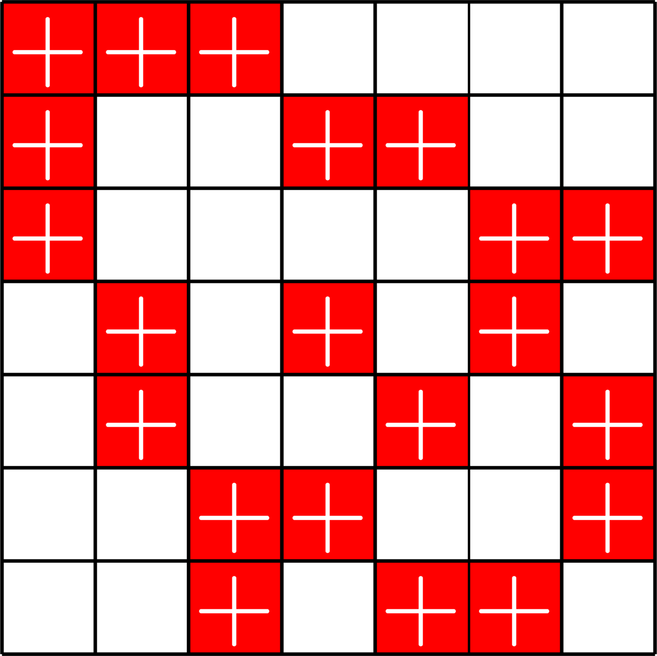

\(=\)
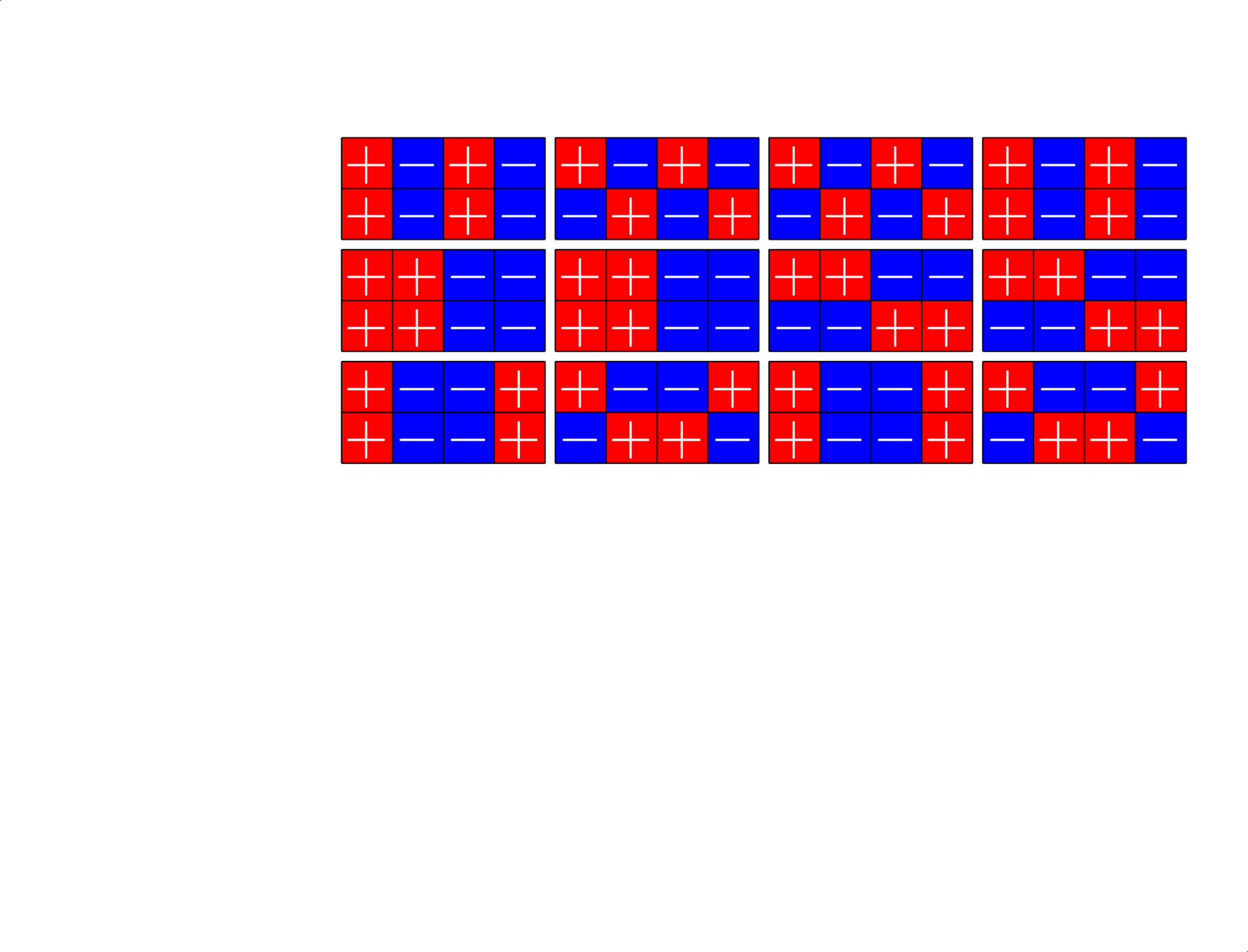
Take a Steiner system with \(r\) ones per column
and an \(r\times (r+1)\) ETF with unimodular entries
The Star product is a "Steiner" ETF

Roadmap for this talk

Compressed Sensing

Vectors that are "Spread out"

Equiangular tight frames
ETFs from groups
\(\Z_{2}\times\Z_{2}\times\Z_{2}\times\Z_{2}\)
The design theory underneath

Real Flat ETFs

Some binary codes
Group divisible designs
ETFs and graphs

Real Flat ETFs

ETFs with all \(\pm 1\) entries: Real Flat ETFs
Why real flat ETFs?
- Waveform design: maximize \(\|x\|_{2}\) subject to \(\|x\|_{\infty}\leq B\) (minimal peak-to-average power ratio)
- Quasi-symmetric designs
- Grey-Rankin equality binary codes
Real Flat ETFs


Real Flat ETFs


\(=\)
Real Flat ETFs

Example. A \(276\times 576\) real ETF

Real Flat ETFs
Theorem (J '13)
\(N\times N\) Hadamard matrix \(\Longrightarrow\) \(N(2N-1)\times 4N^2\) real flat ETF
Previously known real flat ETFs:
- \(N = 2^k\) harmonic ETFs on \(\mathbb{Z}_{2}^{2k+2}\)
- \(N = 6\) [Bracken, McGuire, & Ward, 2006]
Theorem (Mixon, J, Fickus '13)
Real Flat
ETFs
Grey-Rankin
equality
binary codes

1-1 correspondence
We can also construct a real flat \(317886556\times 1907416992\) ETF.


Roadmap for this talk

Compressed Sensing

Vectors that are "Spread out"

Equiangular tight frames
ETFs from groups
\(\Z_{2}\times\Z_{2}\times\Z_{2}\times\Z_{2}\)
The design theory underneath

Real Flat ETFs

Some binary codes
Group divisible designs
ETFs and graphs

Meme of the talk:

\(\mathbb{Z}_{2}\times\mathbb{Z}_{2}\times\mathbb{Z}_{3}\times\mathbb{Z}_{3}\)

Some ETFs
arise from
Spence Difference Sets...
a lot more ETFs
arise from
Group Divisible
Designs!
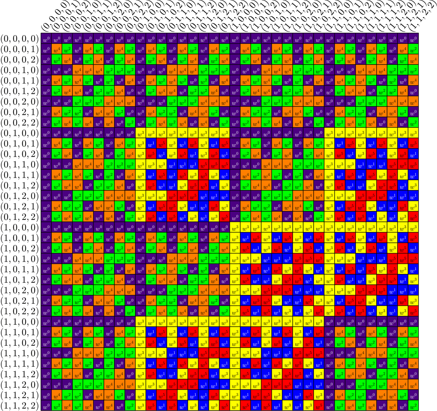
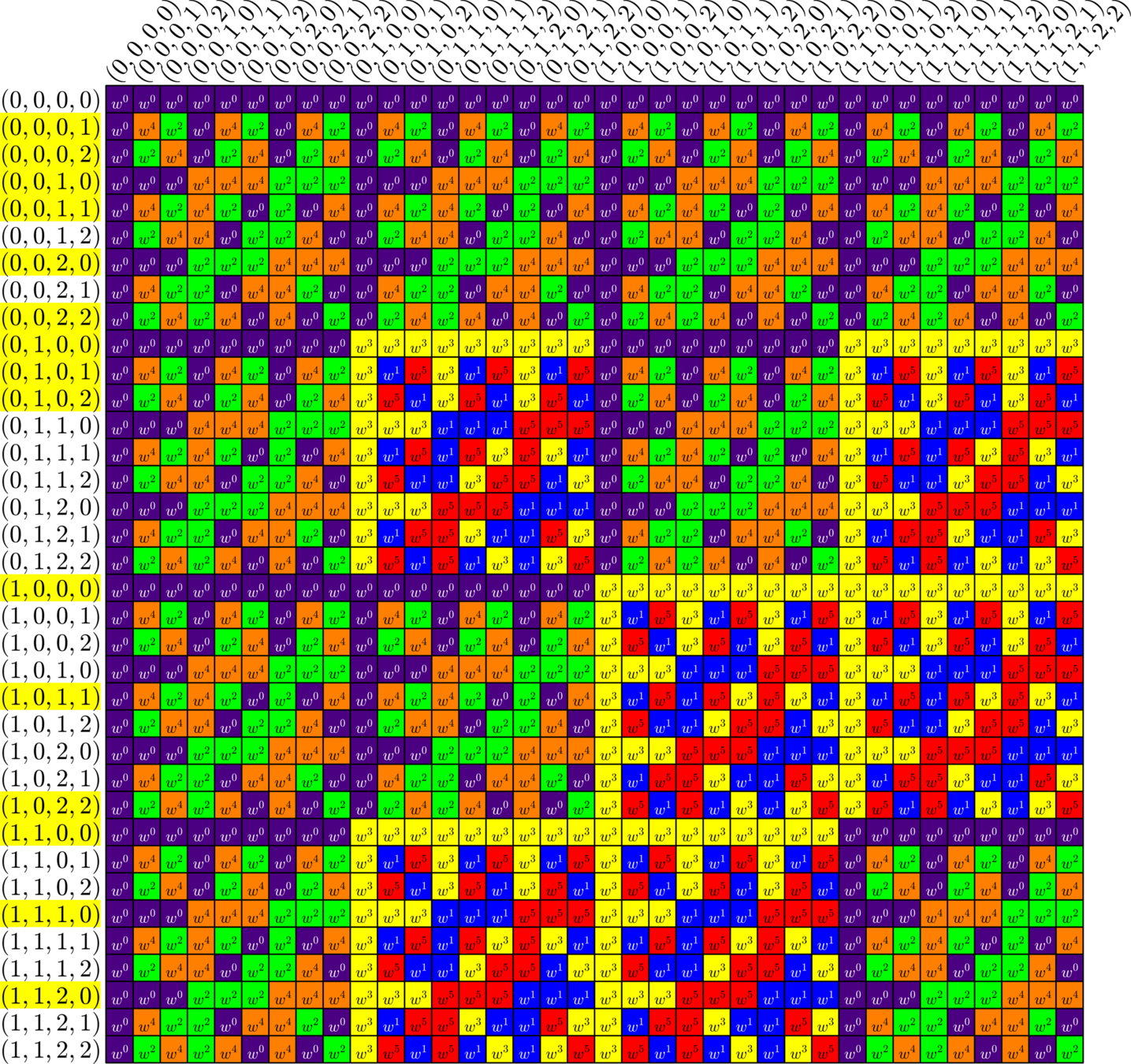

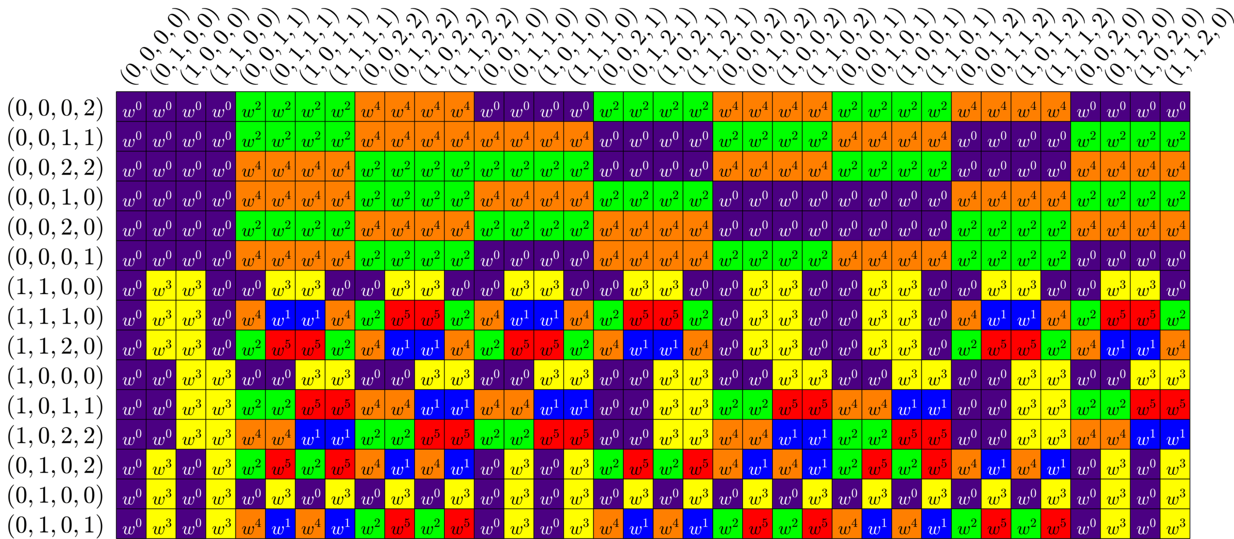
Ex:
\(G\)
\( \mathbb{Z}_{2}\)
\(\times\)
\(\mathbb{Z}_{2}\)
\(\times\)
\(\mathbb{Z}_{3}\)
\(\times\)
\(\mathbb{Z}_{3}\)
\(=\)
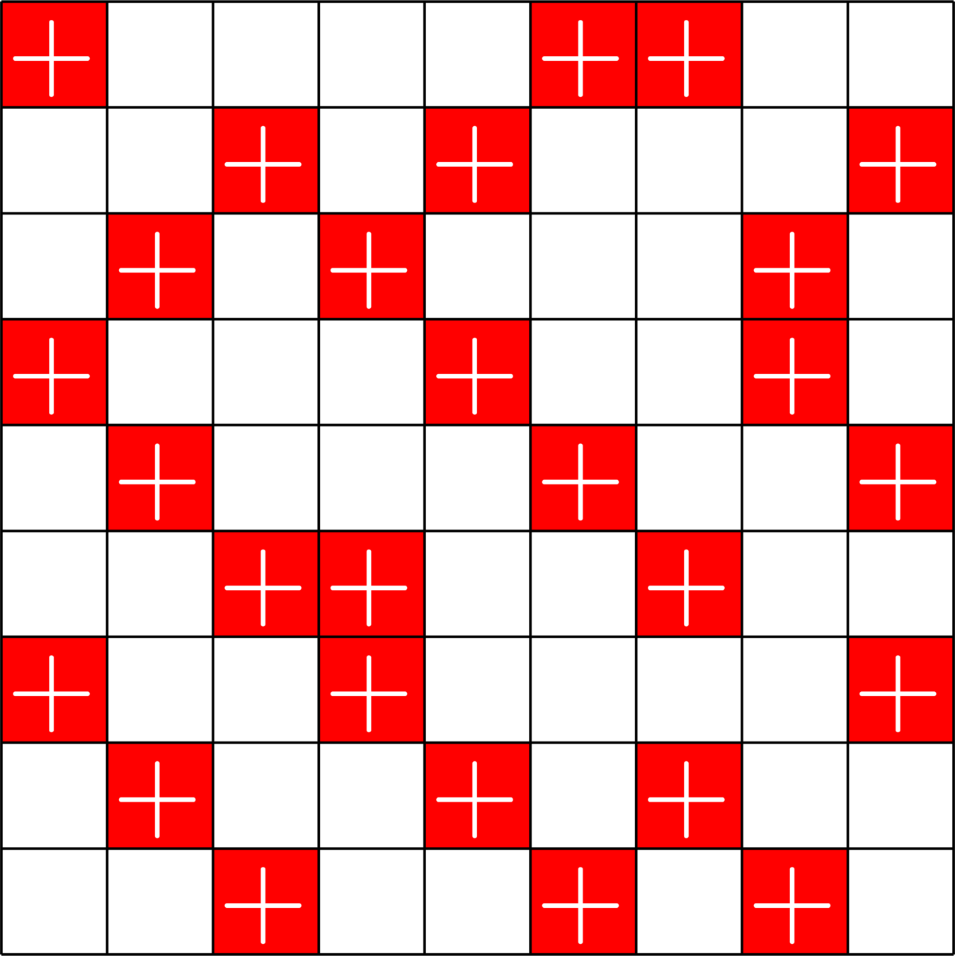
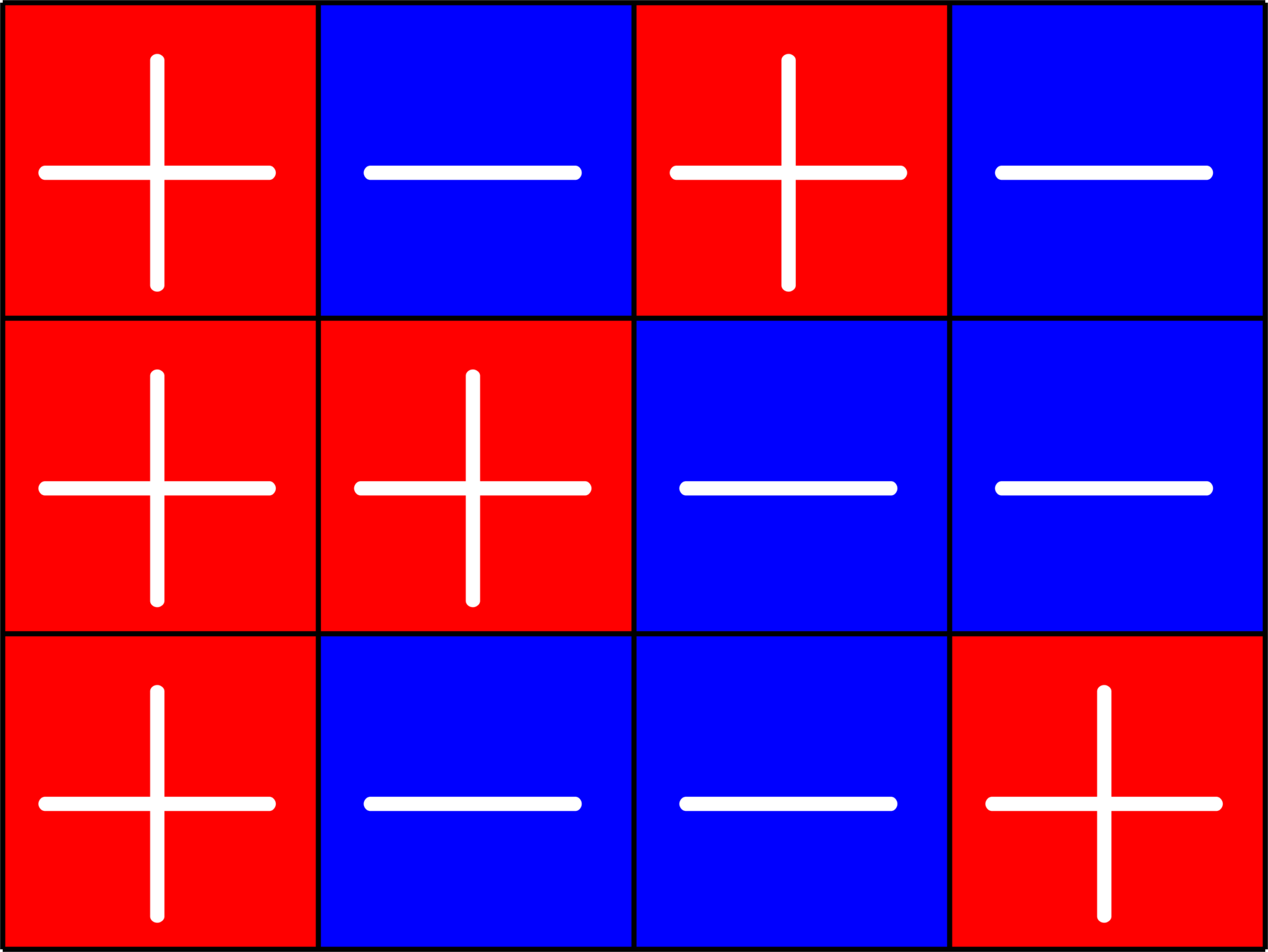

\(\bigotimes\)

\[\left[\begin{array}{l} \\ \\ \\ \\ \\ \\ \\ \\ \\ \\ \\ \end{array}\right.\]
\[\left.\begin{array}{l} \\ \\ \\ \\ \\ \\ \\ \\ \\ \\ \\ \end{array}\right]\]

\[\cong\]
Unitary transformation
\(I_{3}\otimes\)(\(2\times 3\) ETF)
\(3\times 4\) ETF with unimodular entries
???
Group Divisible Designs
Definition. A \(K\)-GDD of type \(M^{U}\) is a \(\{0,1\}\)-matrix \(X\) such that:
- \(X\) has \(UM\) columns.
- Each row of \(X\) has \(K\) ones.
- \(X^{\top}X = R\cdot I_{UM}+J_{UM}-(I_{U}\otimes J_{M})\) for some \(R\in\N\)
Example. The following is a \(3\)-GDD of type \(3^3\):
\(X = \)


\(X^{\top}X = \)
ETFs from GDDs
Theorem (Fickus, J '19). Given a
\(d\times n\) ETF
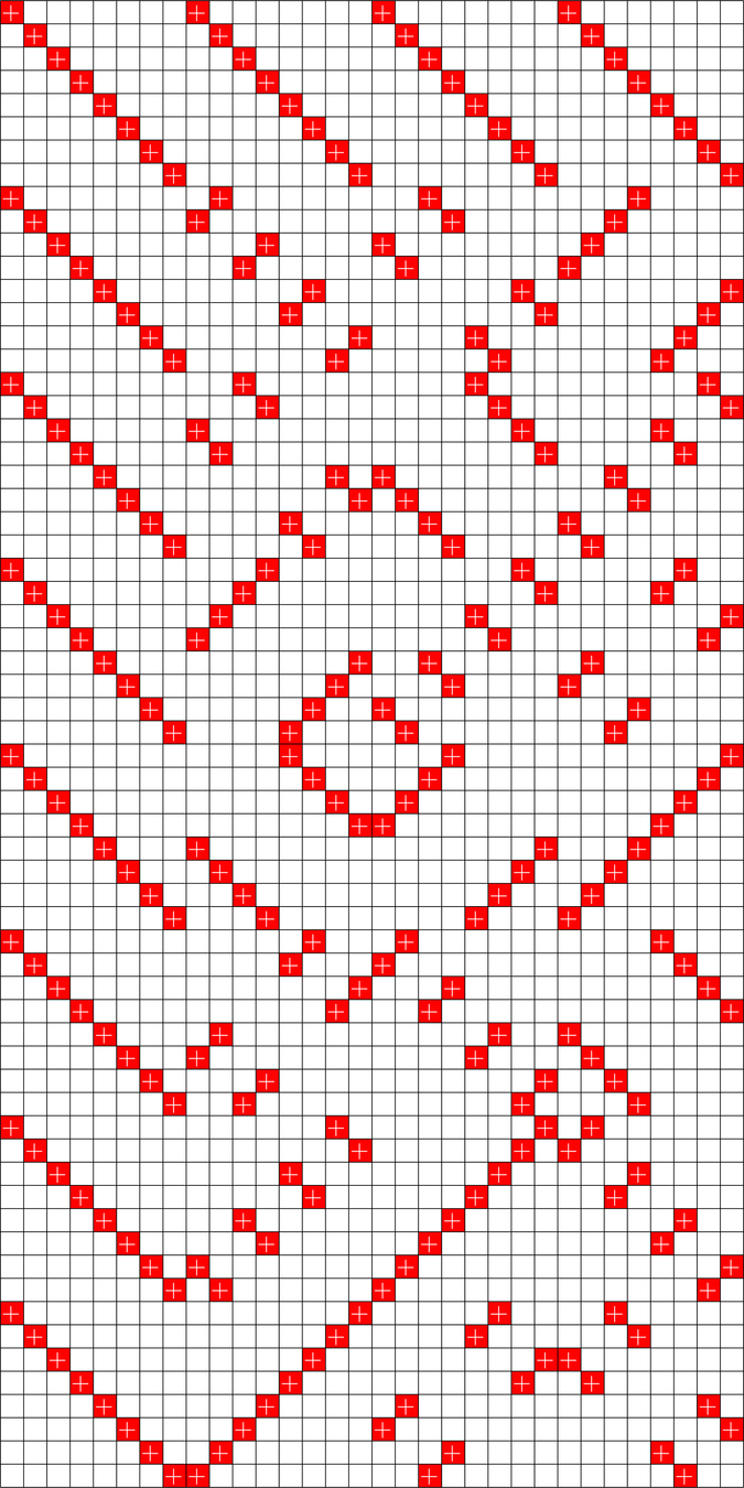
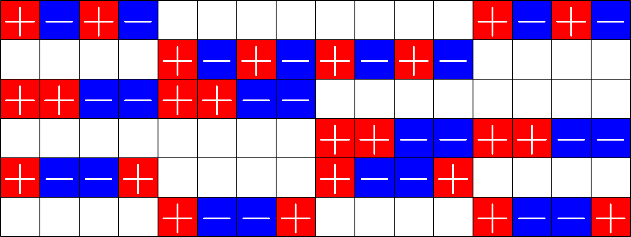
\(k\)-GDD of type \(M^{U}\)
and
provided certain integrality conditions hold, there exists a \(D\times N\) ETF with \(D>d\), \(N>n\) and \(\frac{D}{N}\approx \frac{d}{n}.\)
Real ETFs and Graphs

\(\Phi=\)
- Given a real ETF \(\Phi\)
- Normalize so that all dot products with the first vector are positive.
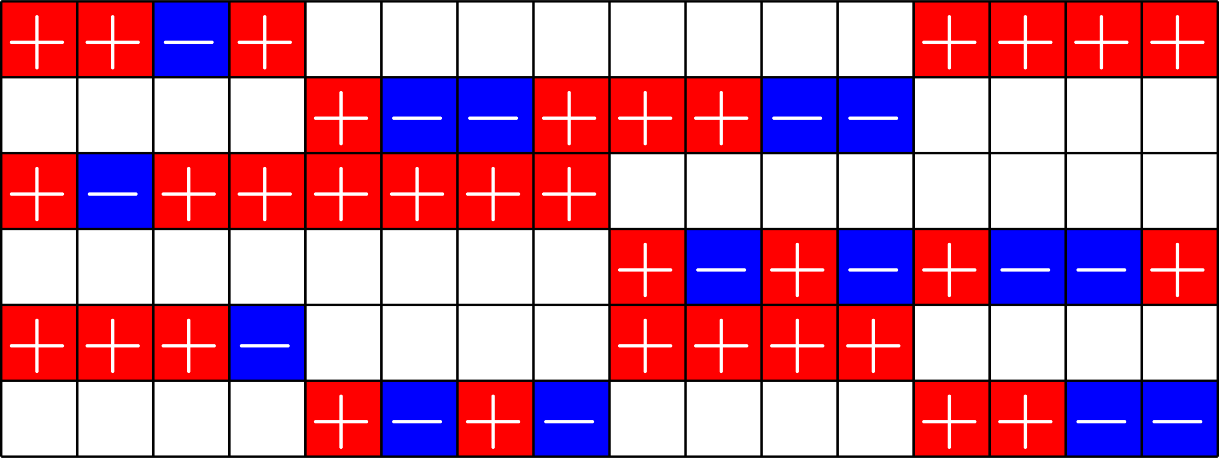
Real ETFs and Graphs
\(\Phi^{\top}\Phi=\)
- Given a real ETF \(\Phi\)
- Normalize so that all dot products with the first vector are positive.
- Look at the gram matrix \(\Phi^{\top}\Phi\)
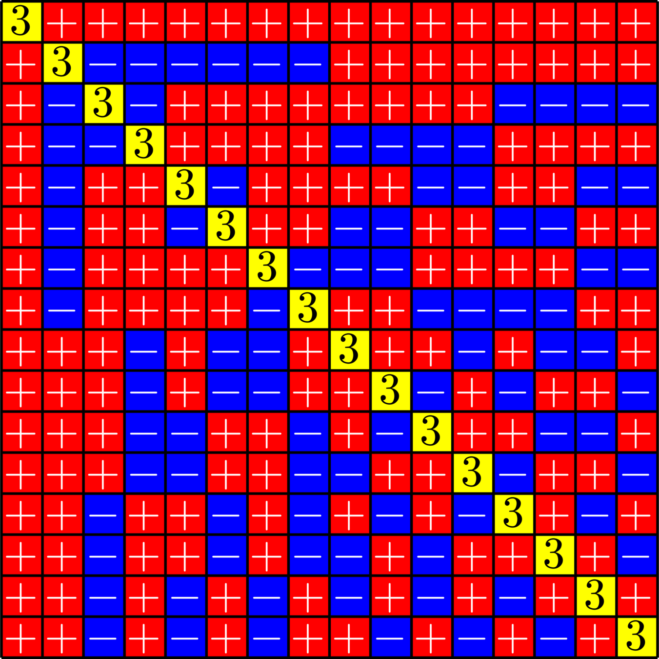
Real ETFs and Graphs
- Given a real ETF \(\Phi\)
- Normalize so that all dot products with the first vector are positive.
- Look at the gram matrix \(\Phi^{\top}\Phi\)
- Remove the first row and column and zero out the diagonal
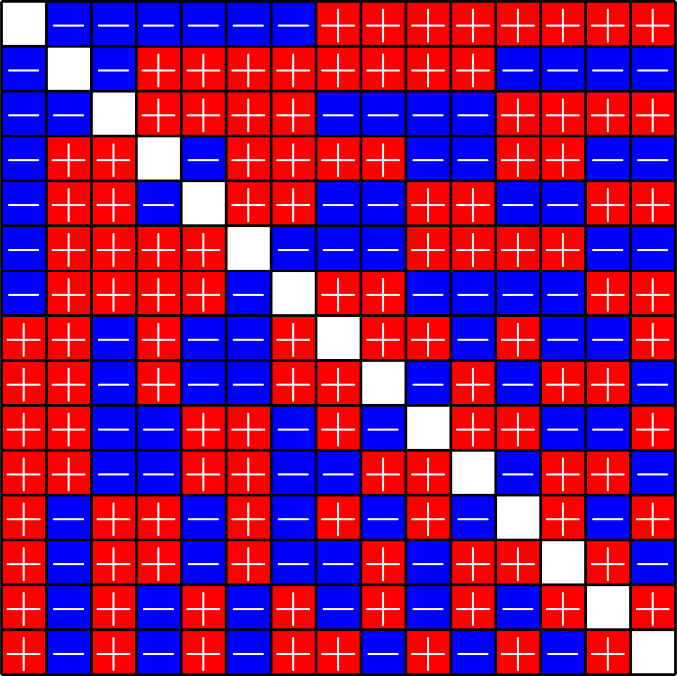
Real ETFs and Graphs
- Given a real ETF \(\Phi\)
- Normalize so that all dot products with the first vector are positive.
- Look at the gram matrix \(\Phi^{\top}\Phi\)
- Remove the first row and column and zero out the diagonal
- This is the Seidel adjacency matrix of a strongly regular graph


Real ETFs and Graphs
A. E. Brouwer maintains a table of known strongly regular graphs.


Our approach:
Real
ETFs


Combinatorial
designs

Strongly
regular graph
Construct
object
Certify
novelty
New Graphs!
Theorem (J, '21). If there exists an
\(h\times h\) Hadamard matrix with \(h\equiv 1\) or \(2\) \(\text{mod}\ 3\),
then there exists a strongly regular graph with parameters:
\[v=h(2h+1),\quad k=h^2-1,\quad \lambda=\frac{1}{2}(h^2-4),\quad \mu = \frac{1}{2}h(h-1)\]


There exists a \(20\times 20\) Hadamard matrix, and hence an SRG(820,399,198,190), which is new!

From Brouwer's table online:
Overall: Five new infinite families!

Roadmap for this talk

Compressed Sensing

Vectors that are "Spread out"

Equiangular tight frames
ETFs from groups
\(\Z_{2}\times\Z_{2}\times\Z_{2}\times\Z_{2}\)
The design theory underneath

Real Flat ETFs

Some binary codes
Group divisible designs
ETFs and graphs

Single-pixel Camera


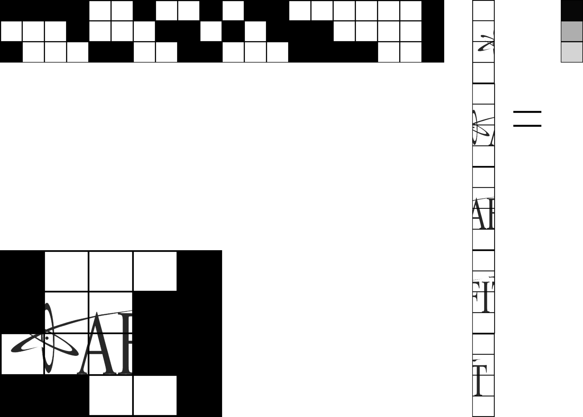


- \(75\times 100\) image \(=7500\) pixels
- We took \(4096\) measurements
Results


- \(75\times 100\) image \(=7500\) pixels
- We took \(4096\) measurements
Results
\(L^{1}\) Minimization Solution
\(L^{2}\) Minimization Solution


Thanks for your attention!
Questions?

Future work:
- Subspaces that are "spread out"
- Frames that saturate the Levenshtein bound
- SRGs from finite geometries
- Diagonals of self-adjoint operators
AFIT Talk
By John Jasper
AFIT Talk
- 700


