Day 30:
PCA and the Pseudoinverse
Theorem. Given an \(m\times n\) matrix \(A\) with singular value decomposition
\[A = \sum_{i=1}^{p}\sigma_{i}u_{i}v_{i}^{\top},\] where \(p=\min\{m,n\},\) fix \(k\leq p\) and define \[A_{k}: = \sum_{i=1}^{k}\sigma_{i}u_{i}v_{i}^{\top}.\] For every \(m\times n\) matrix \(B\) with rank at most \(k\) we have \[\|A-B\|_{F}\geq \|A-A_{k}\|_{F}.\]
Theorem. If \(w_{1},\ldots,w_{n}\) are the columns of \(A\), then \[\|A\|_{F} = \sqrt{\sum_{j=1}^{n}\|w_{j}\|^{2}}\]
Suppose \(A\in\mathbb{R}^{m\times n}\) has singular value decomposition \[A = \sum_{i=1}^{p}\sigma_{i}u_{i}v_{i}^{\top},\] where \(p=\min\{m,n\}.\) In matrix form:
\[A = \left[\begin{array}{cccc} \vert & \vert & & \vert\\ u_{1} & u_{2} & \cdots & u_{m}\\ \vert & \vert & & \vert\end{array}\right] \left[\begin{array}{cccccc} \sigma_{1} & 0 & \cdots & 0 & 0 & \cdots\\ 0 & \sigma_{2} & & 0 & 0 & \cdots\\ \vdots & & \ddots & \vdots & \vdots & \\ 0 & 0 & \cdots & \sigma_{m} & 0 & \cdots\end{array}\right]\left[\begin{array}{ccc} - & v_{1}^{\top} & -\\ - & v_{2}^{\top} & -\\ & \vdots & \\ - & v_{n}^{\top} & -\\ \end{array}\right]\]
\[A = \left[\begin{array}{cccc} \vert & \vert & & \vert\\ u_{1} & u_{2} & \cdots & u_{m}\\ \vert & \vert & & \vert\end{array}\right] \left[\begin{array}{cccc} \sigma_{1} & 0 & \cdots & 0\\ 0 & \sigma_{2} & & 0\\ \vdots & & \ddots & \vdots \\ 0 & 0 & \cdots & \sigma_{m}\\ 0 & 0 & \cdots & 0\\ \vdots & \vdots & & \vdots\end{array}\right]\left[\begin{array}{ccc} - & v_{1}^{\top} & -\\ - & v_{2}^{\top} & -\\ & \vdots & \\ - & v_{n}^{\top} & -\\ \end{array}\right]\]
If \(m<n\)
If \(n<m\)
If \(k\leq p\) and \[A_{k} = \sum_{i=1}^{k}\sigma_{i}u_{i}v_{i}^{\top},\] In matrix form:
\[A = \left[\begin{array}{cccc} \vert & \vert & & \vert\\ u_{1} & u_{2} & \cdots & u_{m}\\ \vert & \vert & & \vert\end{array}\right] \left[\begin{array}{cccccc} \sigma_{1} & 0 & \cdots & 0 & 0 & \cdots\\ 0 & \sigma_{2} & & 0 & 0 & \cdots\\ \vdots & & \ddots & \vdots & \vdots & \\ 0 & 0 & \cdots & \sigma_{k} & 0 & \cdots\\ 0 & 0 & \cdots & 0 & 0 & \\ \vdots & \vdots & & \vdots & & \ddots\end{array}\right]\left[\begin{array}{ccc} - & v_{1}^{\top} & -\\ - & v_{2}^{\top} & -\\ & \vdots & \\ - & v_{n}^{\top} & -\\ \end{array}\right]\]
Corollary. Given an \(m\times n\) matrix \(A\) with singular value decomposition
\[A = \sum_{i=1}^{p}\sigma_{i}u_{i}v_{i}^{\top},\] where \(p=\min\{m,n\},\) fix \(k\leq p\) and define \[A_{k}: = \sum_{i=1}^{k}\sigma_{i}u_{i}v_{i}^{\top}.\]
Let \(a_{1},\ldots,a_{n}\) be the columns of \(A\), let \(a_{1}^{(k)},\ldots,a_{n}^{(k)}\) be the columns of \(A_{k}\). If \(b_{1},\ldots,b_{n}\) are all vectors in some \(k\) dimensional subspace of \(\R^{m}\), then \[\sum_{i=1}^{n}\|a_{i} - a_{i}^{(k)}\|^{2}\leq \sum_{i=1}^{n}\|a_{i} - b_{i}\|^{2}\]
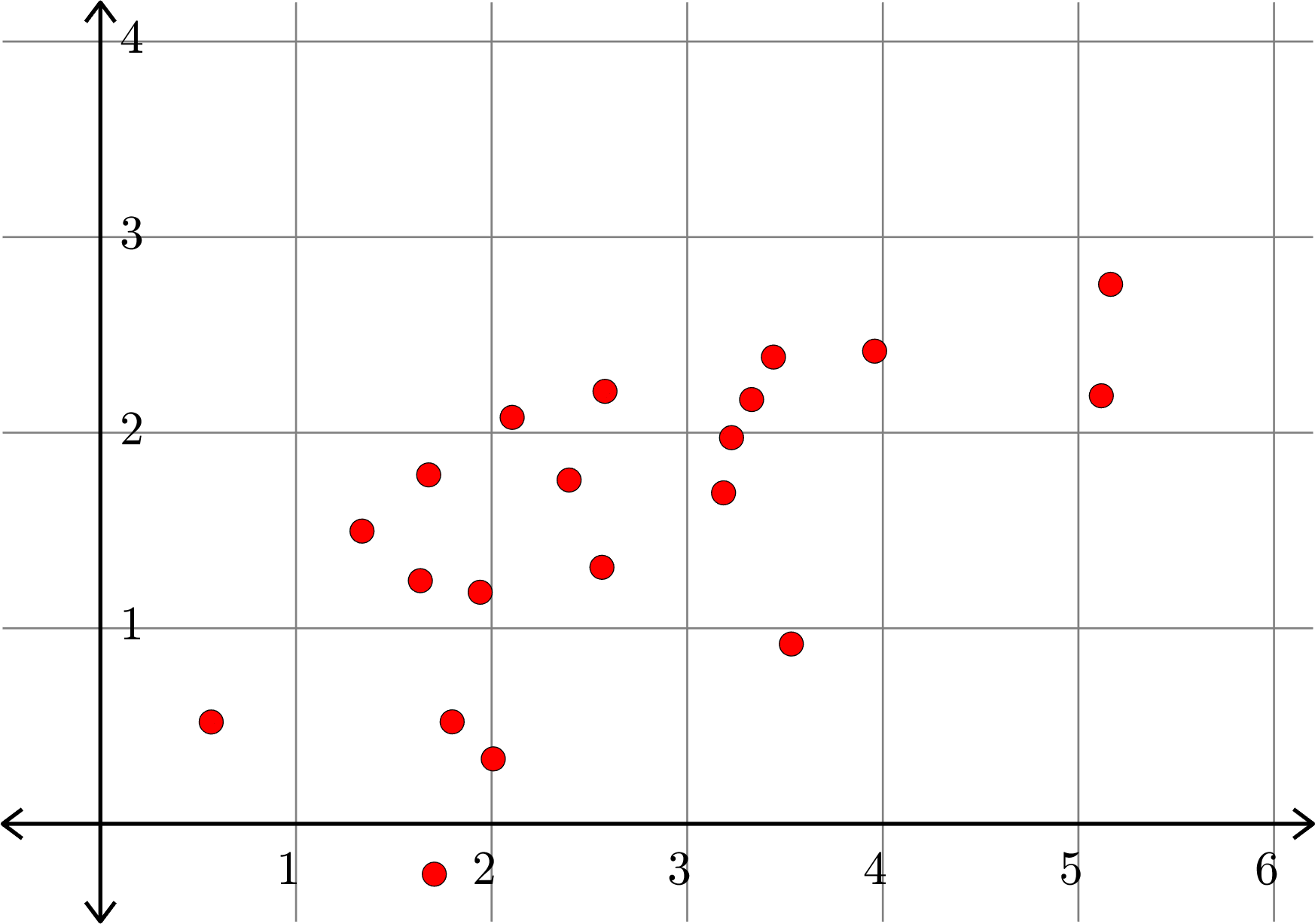
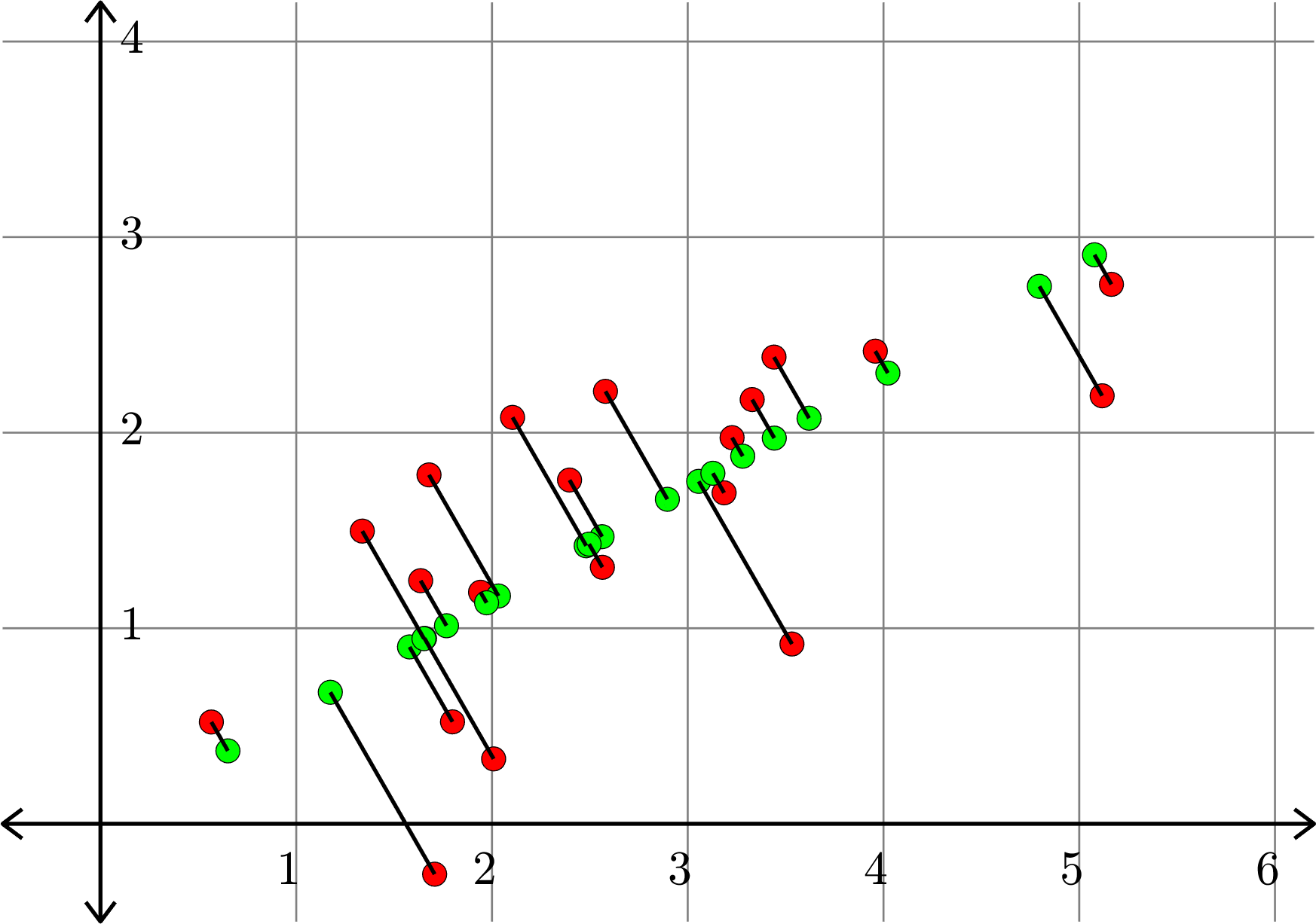
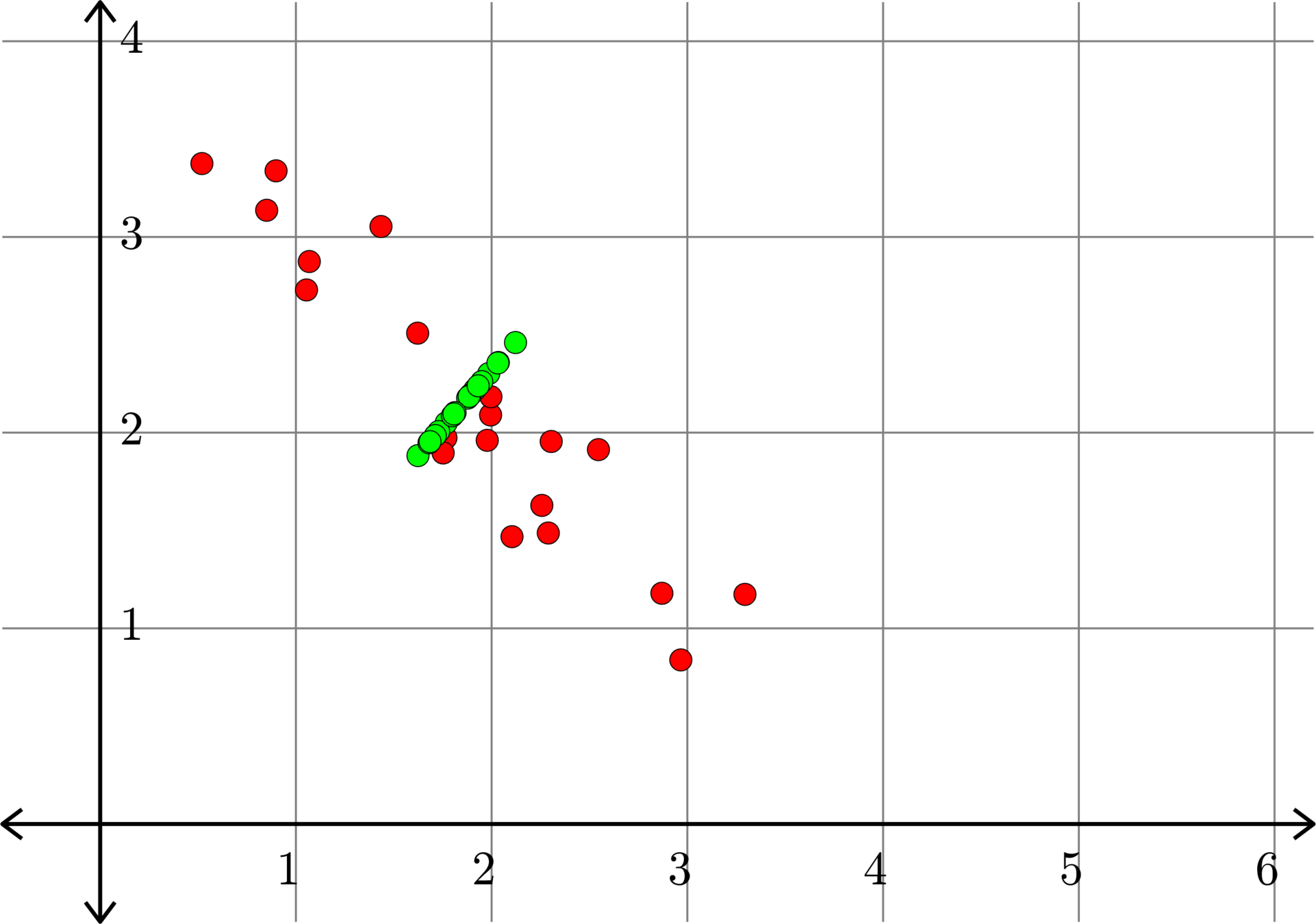
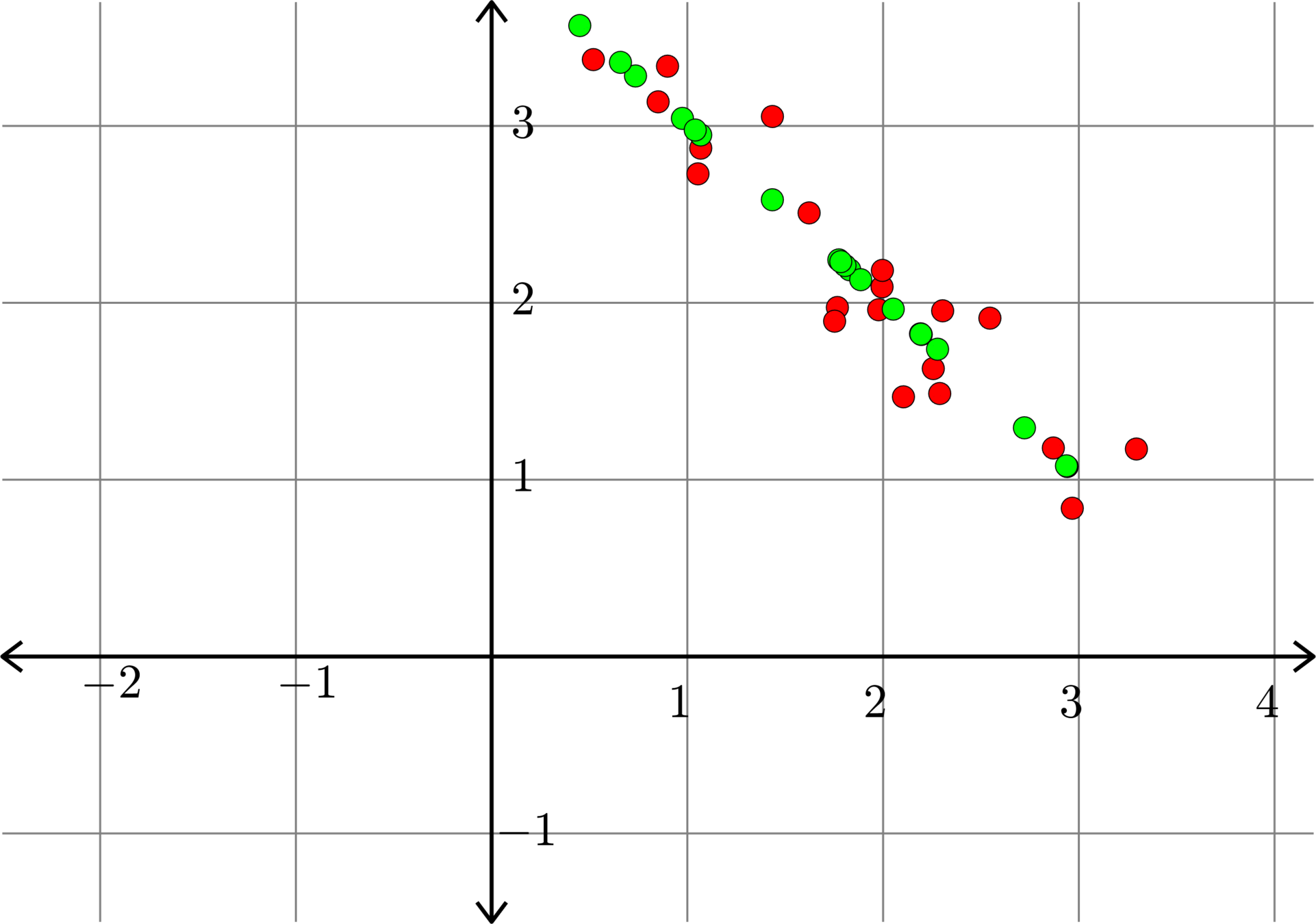
\[A^{\top} = \begin{bmatrix} 1.6356 & 1.2432\\ 3.5324 & 0.9194\\ 5.1171 & 2.1886\\ 1.7070 & -0.2575\\ 2.1051 & 2.0781\\ 3.4407 & 2.3865\\ 2.5796 & 2.2113\\ 2.0085 & 0.3319\\ 3.1858 & 1.6924\\ 3.2266 & 1.9745\\ 2.3962 & 1.7579\\ 5.1645 & 2.7584\\ 2.5640 & 1.3116\\ 3.9581 & 2.4168\\ 1.6782 & 1.7841\\ 1.7983 & 0.5214\\ 0.5665 & 0.5206\\ 3.3292 & 2.1693\\ 1.9416 & 1.1841\\ 1.3375 & 1.4968\\\end{bmatrix}\]
\[A_{1}^{\top} = \begin{bmatrix} 1.7676 & 1.0128\\ 3.0559 & 1.7509\\ 4.7964 & 2.7482\\ 1.1741 & 0.6727\\ 2.4813 & 1.4217\\ 3.6197 & 2.0740\\ 2.8960 & 1.6593\\ 1.6552 & 0.9484\\ 3.1284 & 1.7925\\ 3.2808 & 1.8798\\ 2.5622 & 1.4681\\ 5.0780 & 2.9095\\ 2.4961 & 1.4301\\ 4.0224 & 2.3047\\ 2.0330 & 1.1649\\ 1.5787 & 0.9046\\ 0.6510 & 0.3730\\ 3.4421 & 1.9722\\ 1.9725 & 1.1301\\ 1.6525 & 0.9468 \end{bmatrix}\]
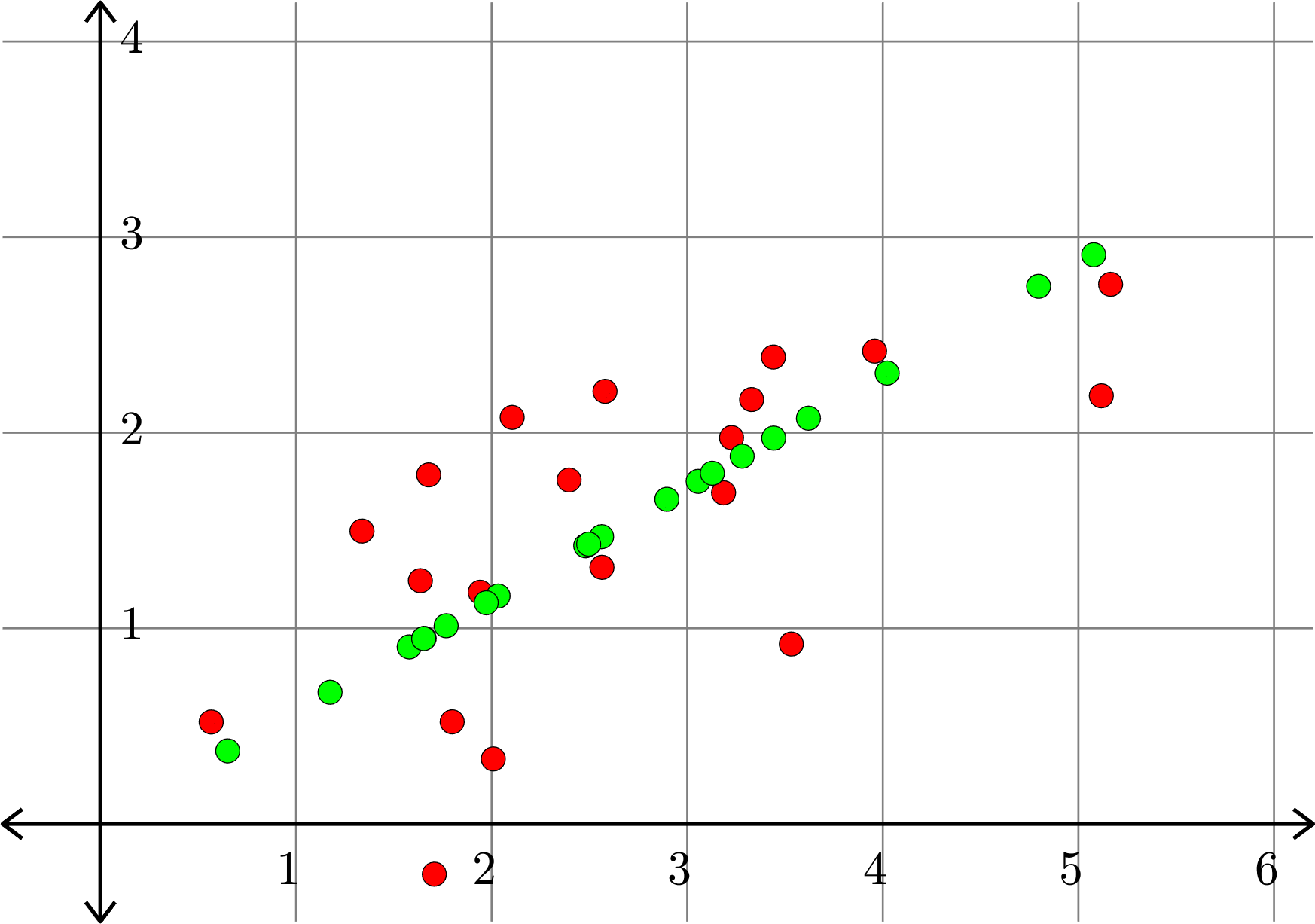
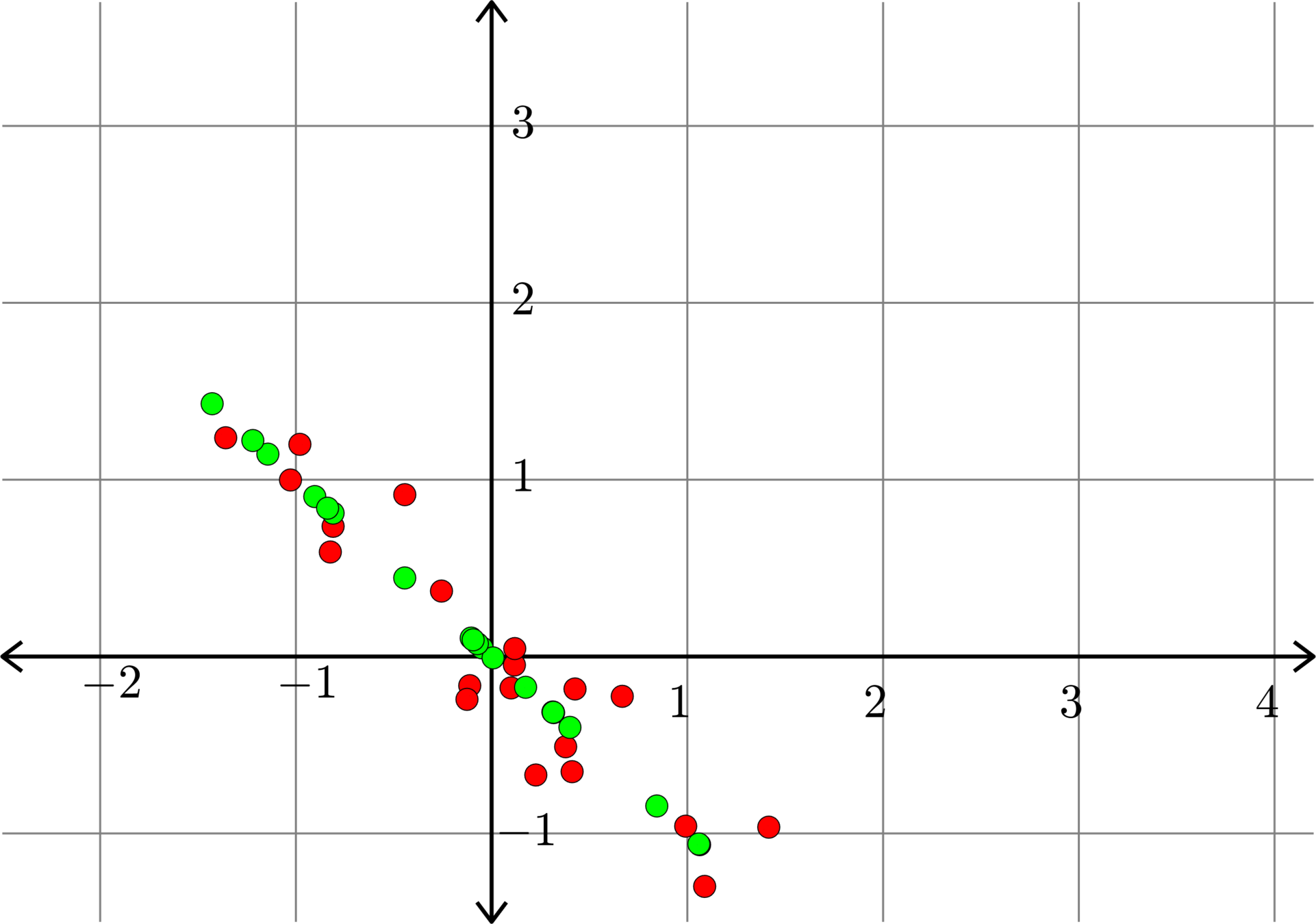
Example.
\(\|A-A_{k}\|_{F} =2.3577... \)
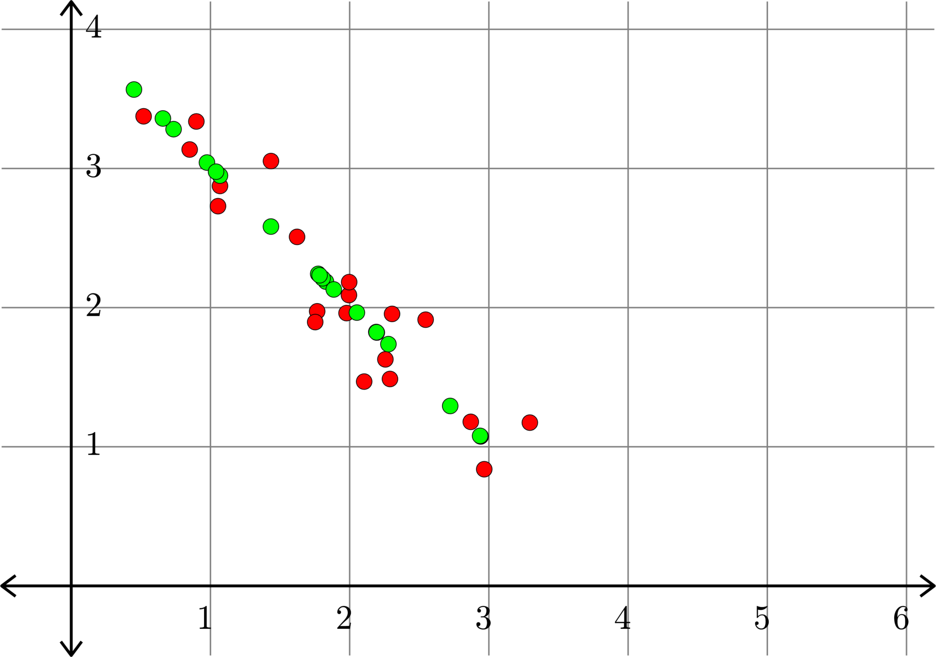
\[A^{\top} = \begin{bmatrix} 1.0684 & 2.8744\\ 0.8506 & 3.1363\\ 2.2565 & 1.6282\\ 2.1041 & 1.4684\\ 2.9667 & 0.8386\\ 1.4346 & 3.0533\\ 1.6221 & 2.5084\\ 1.7665 & 1.9735\\ 0.5197 & 3.3750\\ 1.0541 & 2.7291\\ 0.8986 & 3.3379\\ 1.9947 & 2.0902\\ 3.2943 & 1.1735\\ 2.2895 & 1.4871\\ 1.9775 & 1.9606\\ 2.8699 & 1.1791\\ 2.3043 & 1.9548\\ 2.5457 & 1.9132\\ 1.7523 & 1.8961\\ 1.9964 & 2.1832 \end{bmatrix}\]
Example.
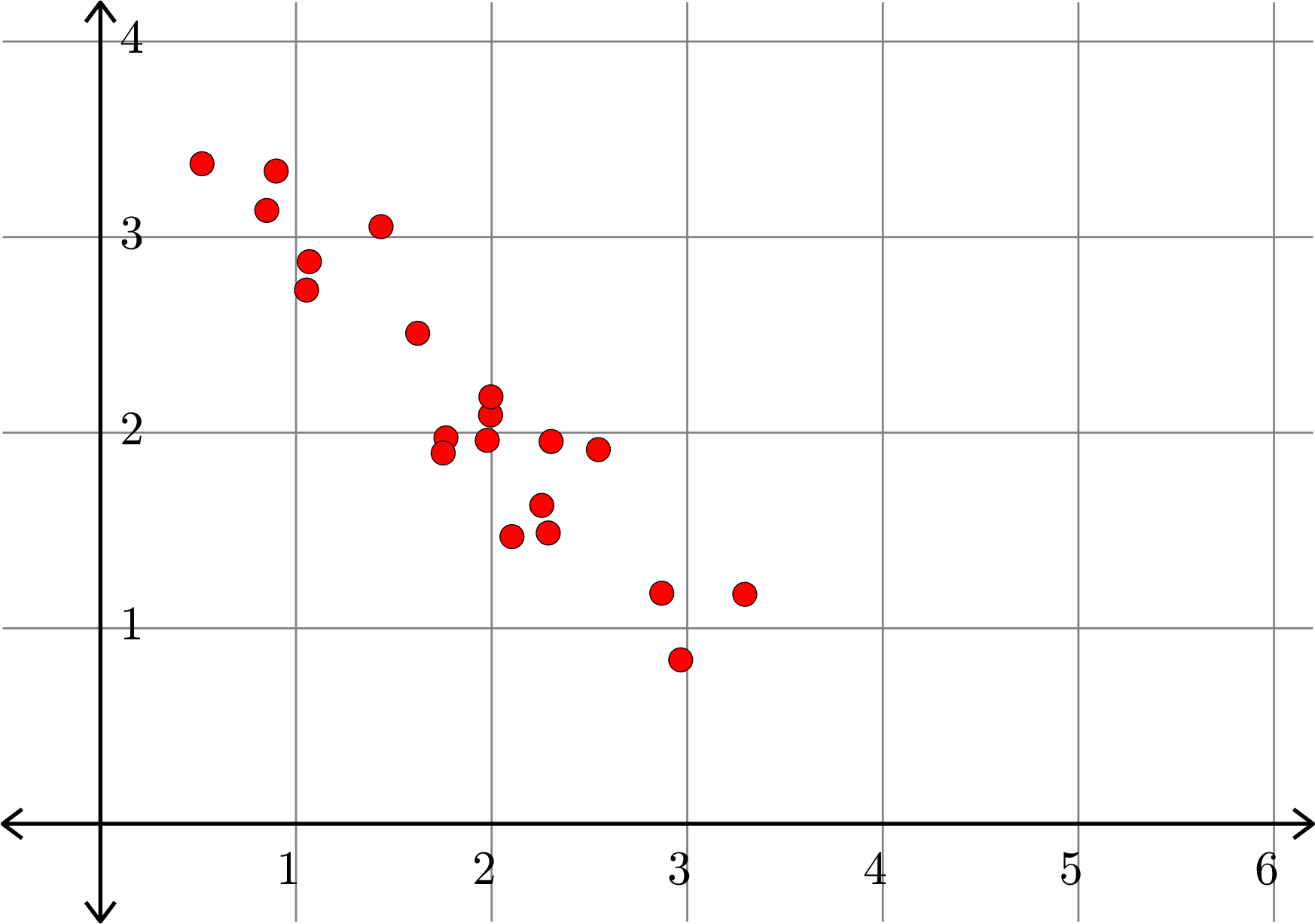
How do we do this?
Principal Component Analysis
Definition. A subset \(X\subset \R^{n}\) is called an affine subspace if there is a subspace \(V\subset \R^{n}\) and a vector \(w\in\R^{n}\) so that
\[X = \{w+v: v\in V\}\]
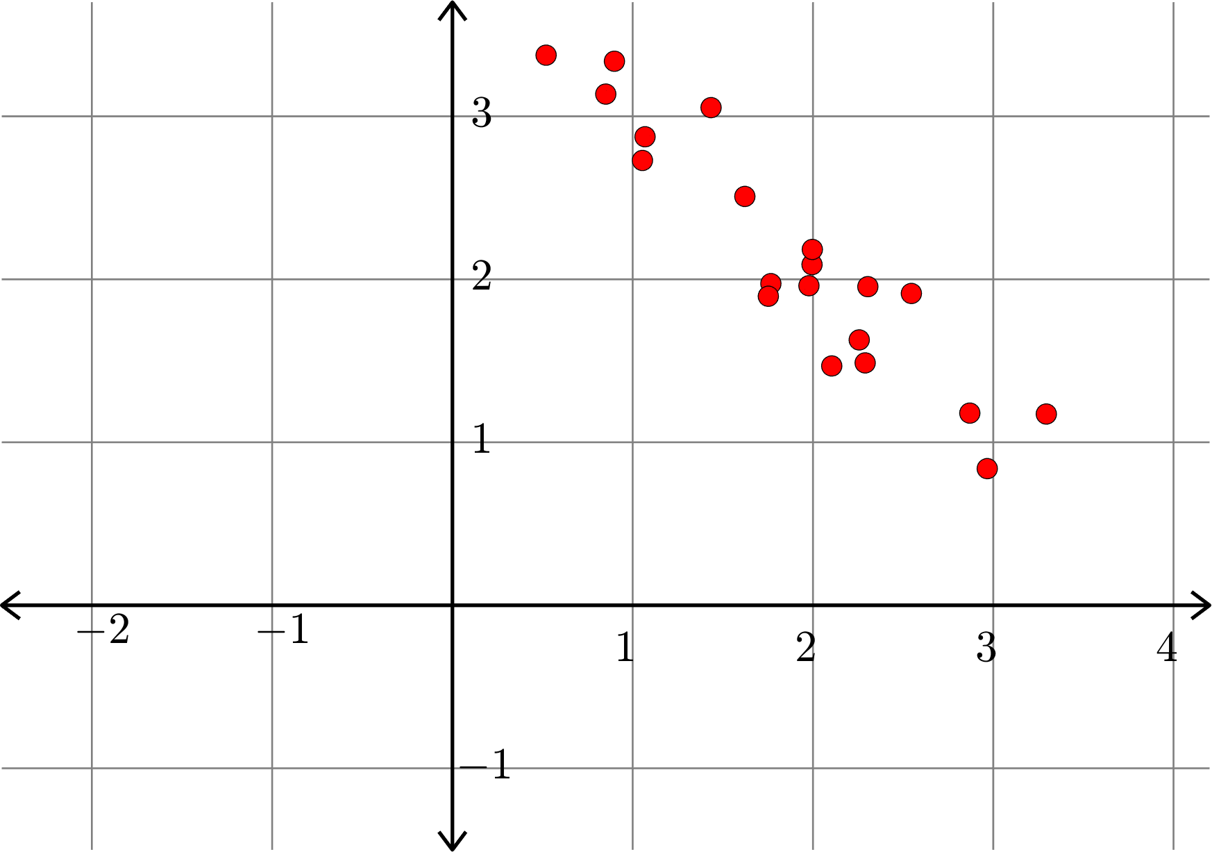
Let \(x_{1},\ldots,x_{n}\) be a collection of vectors in \(\R^{m}.\) Form the matrix
\[A = \begin{bmatrix} | & | & | & & |\\ x_{1} & x_{2} & x_{3} & \cdots & x_{n}\\ | & | & | & & |\end{bmatrix}\]
Define the vector
\[\overline{x} = \frac{1}{n}\left(x_{1}+x_{2}+\cdots+x_{n}\right)\]
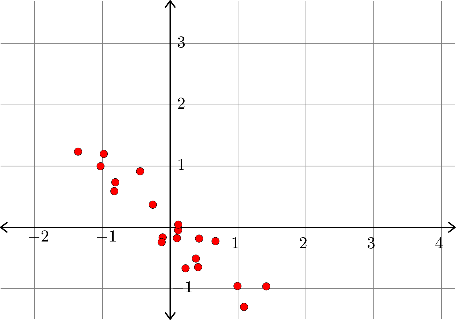
Form the matrix
\[\tilde{A} = \begin{bmatrix} | & | & | & & |\\ (x_{1}-\overline{x}) & (x_{2}-\overline{x}) & (x_{3}-\overline{x}) & \cdots & (x_{n}-\overline{x})\\ | & | & | & & |\end{bmatrix}\]
Principal Component Analysis
Form the matrix
\[\tilde{A}_{k} = \begin{bmatrix} | & | & | & & |\\ y_{1} & y_{2} & y_{3} & \cdots & y_{n}\\ | & | & | & & |\end{bmatrix}\]
The vectors \(y_{1},\ldots,y_{n}\) are in a \(k\)-dimensional subspace \(V\), and
\[\sum_{i=1}^{n}\|(x_{i}-\overline{x})-y_{i}\|^{2}\]
is smallest among all collections of vectors \(y_{1},\ldots,y_{n}\) that live in a \(k\)-dimensional subspace. Note that
\[\sum_{i=1}^{n}\|(x_{i}-\overline{x})-y_{i}\|^{2} = \sum_{i=1}^{n}\|x_{i}-(\overline{x}+y_{i})\|^{2} \]
and the vectors \(\overline{x}+y_{1},\ldots,\overline{x}+y_{n}\) all live in the affine subspace
\[X = \{\overline{x}+v : v\in V\}.\]
Example.
Example.
Example.
Definition. Given an \(m\times n\) matrix \(A\) with singular value decomposition \[A=U\Sigma V^{\top},\] that is, \(U\) and \(V\) are orthogonal matrices, and \(\Sigma\) is an \(m\times n\) diagonal matrix with nonnegative entries \(\sigma_{1}\geq \sigma_{2}\geq \cdots\geq \sigma_{p}\) on the diagonal, we define the pseudoinverse of \(A\) \[A^{+} = V\Sigma^{+}U^{\top}\] where \(\Sigma^{+}\) is the \(n\times m\) diagonal matrix with \(i\)th diagonal entry \(1/\sigma_{i}\) if \(\sigma_{i}\neq 0\) and \(0\) if \(\sigma_{i}=0\).
Example. Consider \[A = \begin{bmatrix} 2 & 0 & 0 & 0\\ 0 & 1 & 0 & 0\\ 0 & 0 & 0 & 0\end{bmatrix}, \quad\text{then}\quad A^{+} = \begin{bmatrix} 1/2 & 0 & 0\\ 0 & 1 & 0\\ 0 & 0 & 0 \\ 0 & 0 & 0 \end{bmatrix}.\]
Example. Consider \[A = \begin{bmatrix} 1 & 0 & 0 & 0\\ 0 & 2 & 0 & 0\\ 0 & 0 & 0 & 0\end{bmatrix}.\]
Then the singular value decomposition of \(A\) is
\[= \begin{bmatrix} 1 & 0 & 0\\ 0 & 1/2 & 0\\ 0 & 0 & 0\\ 0 & 0 & 0\end{bmatrix}.\]
\[A= \begin{bmatrix} 0 & 1 & 0\\ 1 & 0 & 0\\ 0 & 0 & 1\end{bmatrix}\begin{bmatrix} 2 & 0 & 0 & 0\\ 0 & 1 & 0 & 0\\ 0 & 0 & 0 & 0\end{bmatrix}\begin{bmatrix} 0 & 1 & 0 & 0\\ 1 & 0 & 0 & 0\\ 0 & 0 & 1 & 0\\ 0 & 0 & 0 & 1\end{bmatrix}.\]
Hence, the pseudo inverse of \(A\) is
\[A^{+}= \begin{bmatrix} 0 & 1 & 0 & 0\\ 1 & 0 & 0 & 0\\ 0 & 0 & 1 & 0\\ 0 & 0 & 0 & 1\end{bmatrix}\begin{bmatrix} 1/2 & 0 & 0\\ 0 & 1 & 0\\ 0 & 0 & 0\\ 0 & 0 & 0\end{bmatrix}\begin{bmatrix} 0 & 1 & 0\\ 1 & 0 & 0\\ 0 & 0 & 1\end{bmatrix}.\]
Example. Consider \[A = \begin{bmatrix} 1 & 1\\ 1 & 1\end{bmatrix}.\]
Then the singular value decomposition of \(A\) is
\[= \begin{bmatrix}1/4 & 1/4\\ 1/4 & 1/4\end{bmatrix}.\]
\[A= \left(\frac{1}{\sqrt{2}}\begin{bmatrix} 1 & 1\\ 1 & -1\end{bmatrix}\right)\begin{bmatrix} 2 & 0 \\ 0 & 0\end{bmatrix}\left(\frac{1}{\sqrt{2}}\begin{bmatrix} 1 & 1\\ 1 & -1\end{bmatrix}\right).\]
Hence, the pseudo inverse of \(A\) is
\[A^{+}= \left(\frac{1}{\sqrt{2}}\begin{bmatrix} 1 & 1\\ 1 & -1\end{bmatrix}\right)\begin{bmatrix} 1/2 & 0 \\ 0 & 0\end{bmatrix}\left(\frac{1}{\sqrt{2}}\begin{bmatrix} 1 & 1\\ 1 & -1\end{bmatrix}\right).\]
Example. Consider \[B = \begin{bmatrix} 1 & 0 & 1\\ 0 & 1 & 1\end{bmatrix} = \begin{bmatrix} \frac{1}{\sqrt{2}} & \frac{1}{\sqrt{2}}\\[1ex] \frac{1}{\sqrt{2}} & -\frac{1}{\sqrt{2}}\end{bmatrix}\begin{bmatrix} \sqrt{3} & 0 & 0\\ 0 & 1 & 0\end{bmatrix}\begin{bmatrix} \frac{1}{\sqrt{6}} & \frac{1}{\sqrt{6}} & \frac{2}{\sqrt{6}}\\[1ex] \frac{1}{\sqrt{2}} & -\frac{1}{\sqrt{2}} & 0\\[1ex] \frac{1}{\sqrt{3}} & \frac{1}{\sqrt{3}} & -\frac{1}{\sqrt{3}}\end{bmatrix}.\]
Hence, the pseudo inverse of \(B\) is
\[B^{+}=\begin{bmatrix} \frac{1}{\sqrt{6}} & \frac{1}{\sqrt{2}} & \frac{1}{\sqrt{3}}\\[1ex] \frac{1}{\sqrt{6}} & -\frac{1}{\sqrt{2}} & \frac{1}{\sqrt{3}}\\[1ex] \frac{2}{\sqrt{6}} & 0 & -\frac{1}{\sqrt{3}}\end{bmatrix}\begin{bmatrix} 1/\sqrt{3} & 0\\ 0 & 1\\ 0 & 0\end{bmatrix}\begin{bmatrix} \frac{1}{\sqrt{2}} & \frac{1}{\sqrt{2}}\\[1ex] \frac{1}{\sqrt{2}} & -\frac{1}{\sqrt{2}}\end{bmatrix}.\]
\[ = \frac{1}{3}\begin{bmatrix} 2 & -1\\ -1 & 2\\ 1 & 1\end{bmatrix}\]
Note: \[BB^{+} = \begin{bmatrix}1 & 0\\ 0 & 1\end{bmatrix} \quad\text{but}\quad B^{+}B = \frac{1}{3}\begin{bmatrix} 2 & -1 & 1\\ -1 & 2 & 1\\ 1 & 1 & 2\end{bmatrix}\]
Let \(A\) be an \(m\times n\) matrix with singular value decomposition
\[A=U\Sigma V^{\top}.\]
Hence
\[A^{+} = V\Sigma^{+}U^{\top}.\]
Let \(\operatorname{rank}(A)=r\), then
\[\Sigma = \begin{bmatrix} D & \mathbf{0}\\ \mathbf{0} & \mathbf{0}\end{bmatrix}\quad\text{and}\quad \Sigma^{+} = \begin{bmatrix} D^{-1} & \mathbf{0}\\ \mathbf{0}\ & \mathbf{0}\end{bmatrix}\]
where
\[D = \begin{bmatrix}\sigma_{1} & 0 & \cdots & 0\\ 0 & \sigma_{2} & & \vdots\\ \vdots & & \ddots & \vdots\\ 0 &\cdots & \cdots & \sigma_{r} \end{bmatrix}\quad \text{and}\quad D^{-1} = \begin{bmatrix}1/\sigma_{1} & 0 & \cdots & 0\\ 0 & 1/\sigma_{2} & & \vdots\\ \vdots & & \ddots & \vdots\\ 0 &\cdots & \cdots & 1/\sigma_{r} \end{bmatrix}\]
and \(\sigma_{1}\geq \sigma_{2}\geq\ldots\geq \sigma_{r}>0\)
Note: These could be empty matrices.
Using this we have
\[AA^{+}=U\Sigma V^{\top}V\Sigma^{+}U^{\top} = U\Sigma\Sigma^{+}U^{\top} = U \begin{bmatrix} D & \mathbf{0}\\ \mathbf{0} & \mathbf{0}\end{bmatrix}\begin{bmatrix} D^{-1} & \mathbf{0}\\ \mathbf{0} & \mathbf{0}\end{bmatrix}U^{\top}\]
\[= U \begin{bmatrix} I & \mathbf{0}\\ \mathbf{0} & \mathbf{0}\end{bmatrix}U^{\top} = U(\,:\,,1\colon\! r)U(\,:\,,1\colon\! r)^{\top}\]
Orthogonal projection onto \(C(A)\).
\[A^{+}A=V\Sigma^{+}U^{\top} U\Sigma V^{\top}= V\Sigma^{+}\Sigma V^{\top} = V \begin{bmatrix} D^{-1} & \mathbf{0}\\ \mathbf{0} & \mathbf{0}\end{bmatrix}\begin{bmatrix} D & \mathbf{0}\\ \mathbf{0} & \mathbf{0}\end{bmatrix}V^{\top}\]
\[= V \begin{bmatrix} I & \mathbf{0}\\ \mathbf{0} & \mathbf{0}\end{bmatrix}V^{\top} = V(\,:\,,1\colon\! r)V(\,:\,,1\colon\! r)^{\top}\]
Orthogonal projection onto ???.
If \(A\) has singular value decomposition
\[A=U\Sigma V^{\top},\]
then
\[A^{\top} = (U\Sigma V^{\top})^{\top} = V\Sigma^{\top} U^{\top}.\]
From this we see:
- The singular values of \(A\) and \(A^{\top}\) are the same.
- The vector \(v\) is a right singular vector of \(A\) if and only if \(v\) is a left singular vector of \(A^{\top}\).
- The vector \(u\) is a left singular vector of \(A\) if and only if \(u\) is a right singular vector of \(A^{\top}\).
- If \(A\) is rank \(r\), then the first \(r\) columns of \(V\) are an orthonormal basis for \(C(A^{\top})\).
\[A^{+}A = V(\,:\,,1\colon\! r)V(\,:\,,1\colon\! r)^{\top}\]
Orthogonal projection onto \(C(A^{\top})\).
Example. Consider the equation
\[\begin{bmatrix}1 & 1\\ 1 & 2\\ 1 & 3\end{bmatrix}\begin{bmatrix}x_{1}\\ x_{2}\end{bmatrix} = \begin{bmatrix}1\\ 4\\ 9\end{bmatrix}.\]
This is an example of an overdetermined system (more equations than unknowns). Note that this equation has no solution since
\[\text{rref}\left(\begin{bmatrix}1 & 1 & 1\\ 1 & 2 & 4\\ 1 & 3 & 9\end{bmatrix}\right) = \begin{bmatrix} 1 & 0 & 0\\ 0 & 1 & 0\\ 0 & 0 & 1\end{bmatrix}\]
What if we want to find the vector \(\hat{x} = [x_{1}\ x_{2}]^{\top}\) that is closest to being a solution, that is, \(\hat{x}\) is the vector so that \(\|A\hat{x}-b\|\) is as small as possible. This is called the least squares solution to the above equation.
Now, consider a general matrix equation:
\[Ax=b.\]
- The closest point in \(C(A)\) to \(b\) is \(AA^{+}b\), since \(AA^{+}\) is the orthogonal projection onto \(C(A)\).
- Take \(\hat{x} = A^{+}b\), then we have \[A\hat{x} = AA^{+}b\]
- So \(\hat{x} = A^{+}b\) is a least squares solution to \(Ax=b\).
Note: If \(Ax=b\) has a solution, that is, \(b\in C(A)\), then \(\hat{x}\) is a solution to \(Ax=b\), since \(AA^{+}b=b\).
Example. Consider \[A= \begin{bmatrix} 1 & 0 \\ 0 & 1 \\ 1 & 1\end{bmatrix} = \begin{bmatrix} \frac{1}{\sqrt{6}} & \frac{1}{\sqrt{2}} & \frac{1}{\sqrt{3}}\\[1ex] \frac{1}{\sqrt{6}} & -\frac{1}{\sqrt{2}} & \frac{1}{\sqrt{3}}\\[1ex] \frac{2}{\sqrt{6}} & 0 & -\frac{1}{\sqrt{3}}\end{bmatrix}\begin{bmatrix} \sqrt{3} & 0\\ 0 & 1\\ 0 & 0\end{bmatrix}\begin{bmatrix} \frac{1}{\sqrt{2}} & \frac{1}{\sqrt{2}}\\[1ex] \frac{1}{\sqrt{2}} & -\frac{1}{\sqrt{2}}\end{bmatrix}.\]
Then, \[A^{+} = \begin{bmatrix} 1 & 0 & 1\\ 0 & 1 & 1\end{bmatrix} = \begin{bmatrix} \frac{1}{\sqrt{2}} & \frac{1}{\sqrt{2}}\\[1ex] \frac{1}{\sqrt{2}} & -\frac{1}{\sqrt{2}}\end{bmatrix}\begin{bmatrix} 1/\sqrt{3} & 0 & 0\\ 0 & 1 & 0\end{bmatrix}\begin{bmatrix} \frac{1}{\sqrt{6}} & \frac{1}{\sqrt{6}} & \frac{2}{\sqrt{6}}\\[1ex] \frac{1}{\sqrt{2}} & -\frac{1}{\sqrt{2}} & 0\\[1ex] \frac{1}{\sqrt{3}} & \frac{1}{\sqrt{3}} & -\frac{1}{\sqrt{3}}\end{bmatrix}.\]
\[ = \frac{1}{3}\begin{bmatrix} 2 & -1 & 1\\ -1 & 2 & 1\end{bmatrix}\]
If we take \(b=[1\ \ 1\ \ 1]^{\top}\), then the equation \(Ax=b\) has no solution. However, the least squares solution is
\[\hat{x} = A^{+}\begin{bmatrix}1\\1\\1\end{bmatrix} = \begin{bmatrix}2/3\\ 2/3\end{bmatrix}.\]
Linear Algebra Day 30
By John Jasper


