Equiangular tight frames:
From algebraic tyranny to combinatorial freedom
John Jasper
Air Force Institute of Technology
Rocky Mountain Algebraic Combinatorics Seminar
The views expressed in this talk are those of the speaker and do not reflect the official policy
or position of the United States Air Force, Department of Defense, or the U.S. Government.
https://slides.com/johnjasper/rmacs1/

A Toy Packing Problem
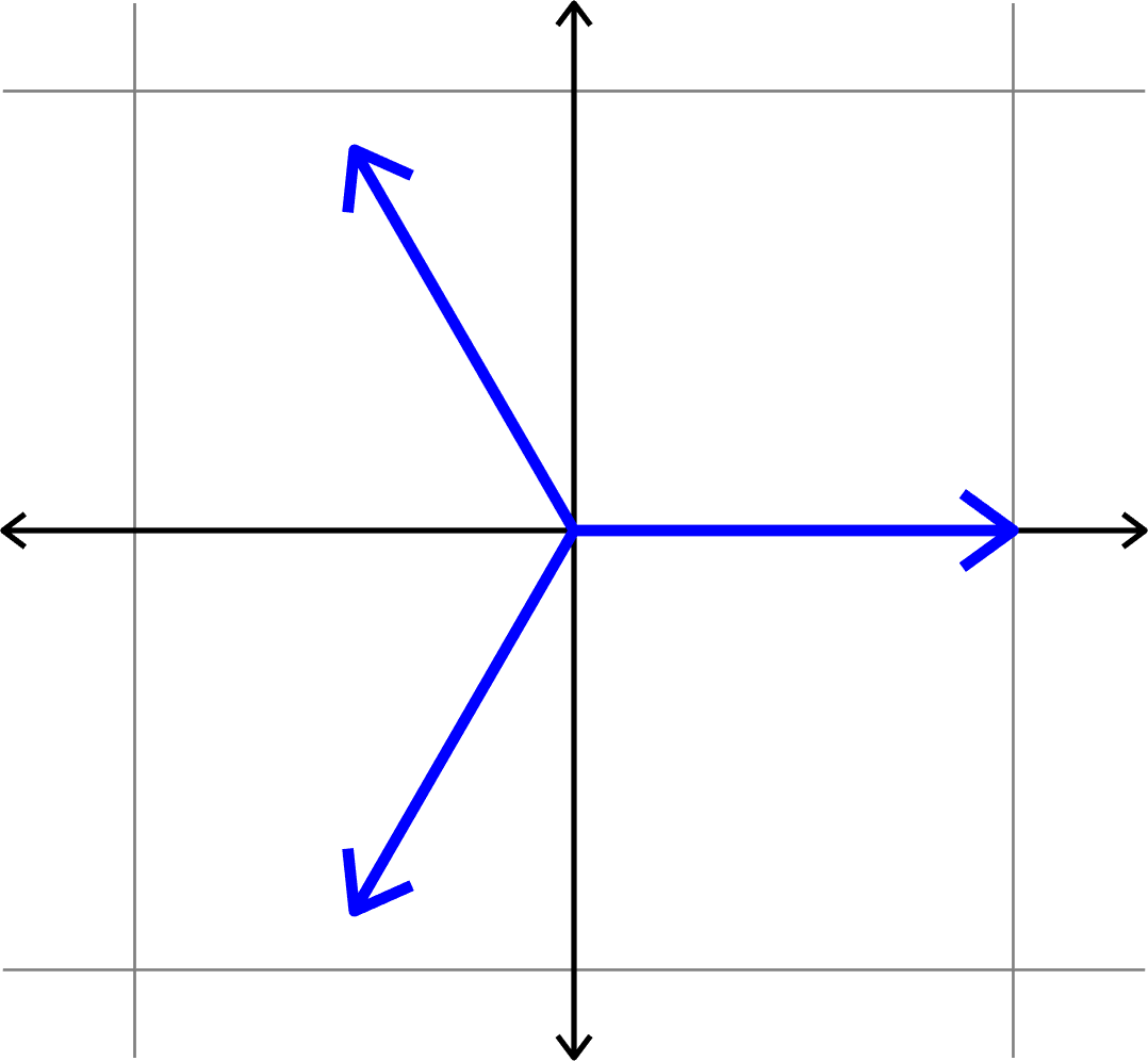
Want: \(N\) points maximally "spread out"
Distance: \(d(x,y) = \) min. arc length

Spread out: maximize min. distance
Want: \(N\) points maximally "spread out"
Distance: \(d(x,y) = \) min. arc length

Some solutions:
\(N=2\)
\(N=3\)
\(N=4\)
\(N=5\)


A Toy Packing Problem
Spread out: maximize min. distance
How do we know these are optimal?
Take pts \(\{x_{1},\ldots,x_{N}\}\) arranged counterclockwise
\(\theta_{n}=\) arclength from \(x_{n}\) to \(x_{n+1}\)
\[\min_{n\neq m}d(x_{n},x_{m})\]
\[\leq \min_{n}\theta_{n}\]
\[\leq \frac{1}{N}\sum_{n=1}^{N}\theta_{n}\]
\[= \frac{2\pi}{N}\]


A Toy Packing Problem
\[\min_{n\neq m}d(x_{n},x_{m})\leq \frac{2\pi}{N}\]

Bound:

A Toy Packing Problem

\(N=5\)
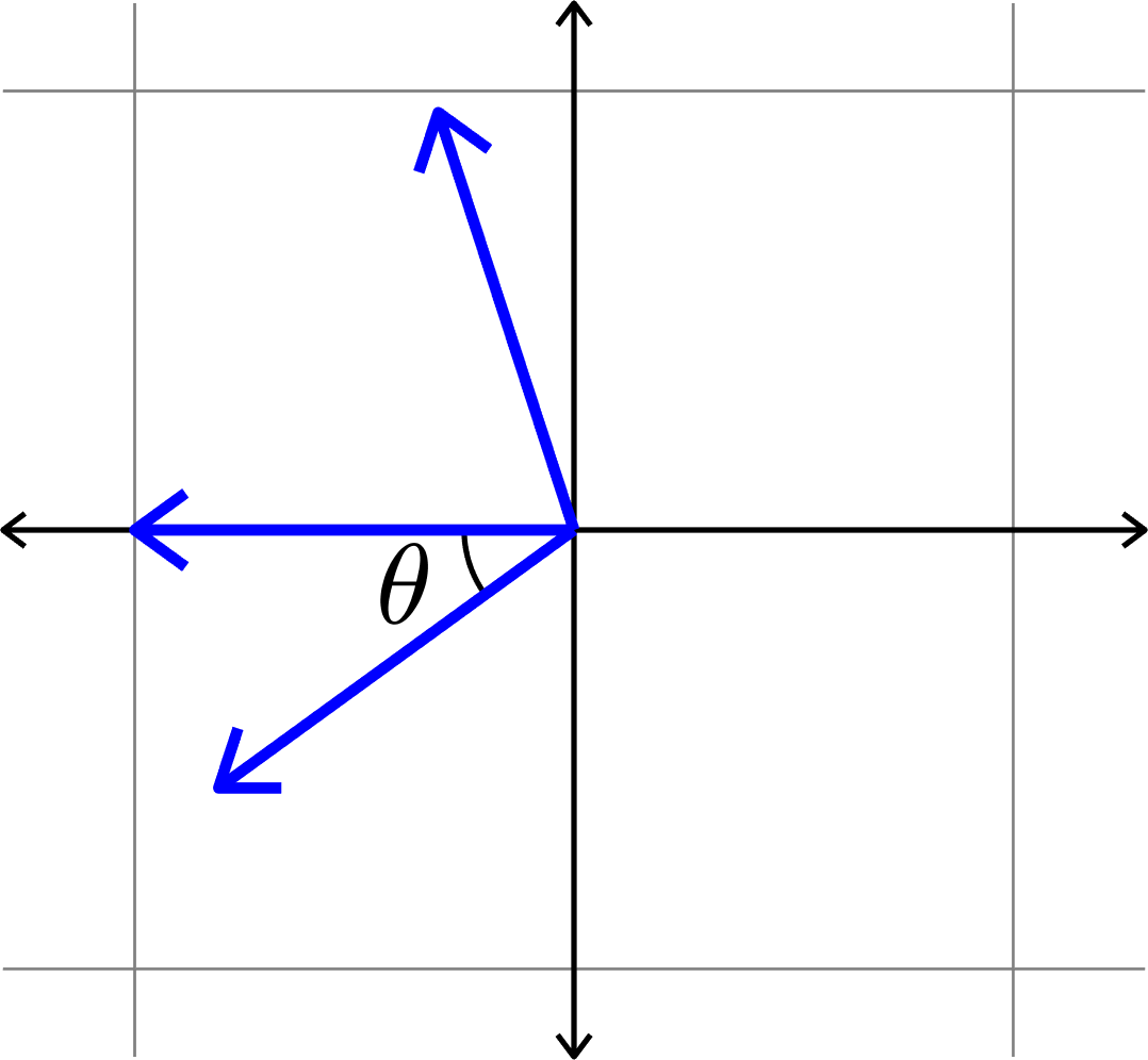
Definition. Given unit vectors \(\Phi=(\varphi_{i})_{i=1}^{N}\), we define the coherence
\[\mu(\Phi) = \max_{i\neq j}|\langle \varphi_{i},\varphi_{j}\rangle|.\]
Measuring how "spread out" vectors are
\[\mu(\Phi) = \cos(\theta)\]
\(\mu(\Phi) = \cos(\theta)\)??

\(\mu(\Phi) = \cos(\theta)\)
Measuring how "spread out" vectors are
Definition. Given unit vectors \(\Phi=(\varphi_{i})_{i=1}^{N}\), we define the coherence
\[\mu(\Phi) = \max_{i\neq j}|\langle \varphi_{i},\varphi_{j}\rangle|.\]
Measuring how "spread out" vectors are
Definition. Given unit vectors \(\Phi=(\varphi_{i})_{i=1}^{N}\), we define the coherence
\[\mu(\Phi) = \max_{i\neq j}|\langle \varphi_{i},\varphi_{j}\rangle|.\]
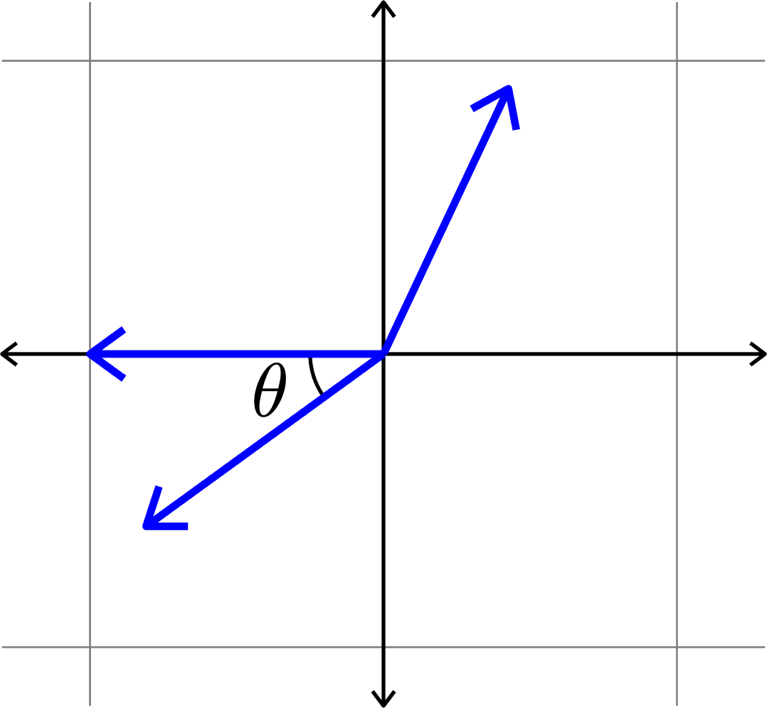
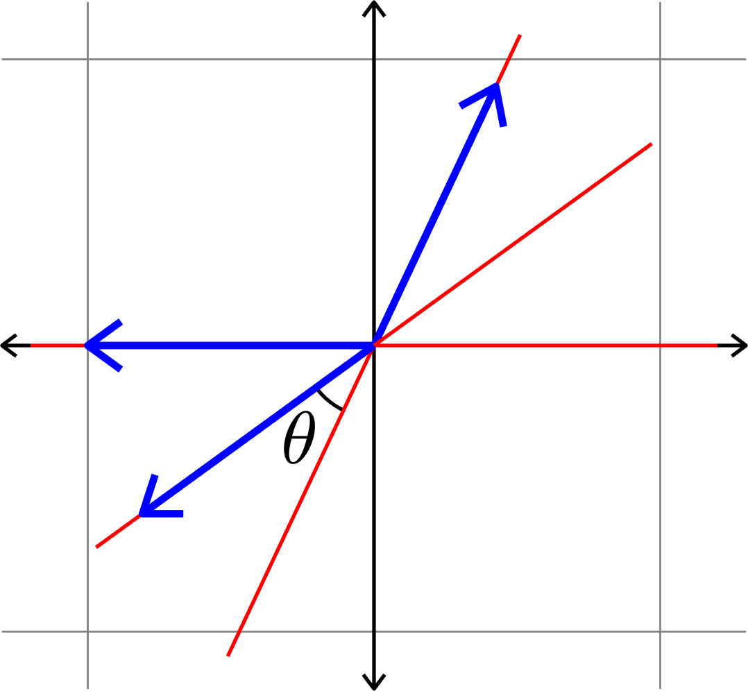
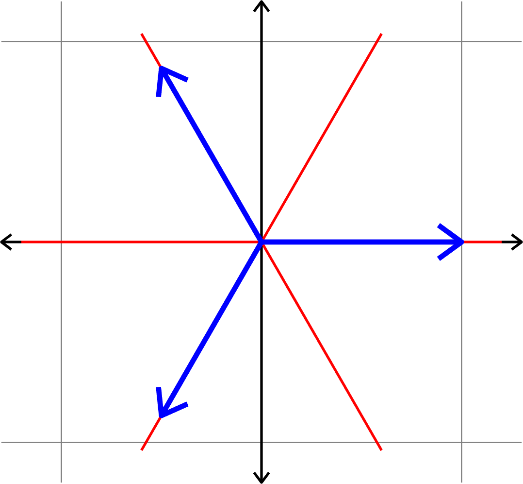
Minimizing coherence
between vectors
\(\Updownarrow\)
Maximizing min. angle
between lines

Example.
Measuring how "spread out" vectors are
Definition. Given unit vectors \(\Phi=(\varphi_{i})_{i=1}^{N}\), we define the coherence
\[\mu(\Phi) = \max_{i\neq j}|\langle \varphi_{i},\varphi_{j}\rangle|.\]
Given \((d,N)\) find \(\Phi = (\varphi_{i})_{i=1}^{N}\subset\mathbb{R}^{d}\) such that \(\mu(\Phi)\) is minimal.
Goal:
Roadmap for this talk
Packing points
Vectors that are "Spread out"
Equiangular tight frames
ETFs from groups
\(\Z_{2}\times\Z_{2}\times\Z_{2}\times\Z_{2}\)
The design theory underneath

Real Flat ETFs

Some binary codes
Group divisible designs
ETFs and graphs

Vectors that are as spread out as possible
Theorem (the Welch bound). Given a collection of unit vectors
\(\Phi=(\varphi_{i})_{i=1}^{N}\) in \(\mathbb{C}^d\), the coherence satisfies
\[\mu(\Phi)\geq \sqrt{\frac{N-d}{d(N-1)}}.\]
Equality holds if and only if the following two conditions hold:
- Tight: There is a constant \(A>0\) such that \[\sum_{i=1}^{N}|\langle v,\varphi_{i}\rangle|^{2} = A\|v\|^{2} \quad\text{for all } v.\]
- Equiangular: There is a constant \(\alpha\) such that \[|\langle\varphi_{i},\varphi_{j}\rangle| = \alpha\quad\text{for all }i\neq j.\]
Welch bound equality \(\Longleftrightarrow\) equiangular tight frame (ETF)
Tightness and short, fat matrices
Useful matrix representation: \(\quad\Phi = \begin{bmatrix} | & | & & |\\ \varphi_{1} & \varphi_{2} & \cdots & \varphi_{N}\\ | & | & & |\end{bmatrix}\)
Tightness: There is a constant \(A>0\) such that \[\sum_{i=1}^{N}|\langle v,\varphi_{i}\rangle|^{2} = A\|v\|^{2} \quad\text{for all } v.\]

( )
\(\Leftrightarrow\quad\Phi\Phi^{\ast} = AI\)
\(\Leftrightarrow\quad\) the rows of \(\Phi\) are orthogonal and equal norm
\(\langle v,\Phi\Phi^{\ast}v\rangle = \)
\(\langle v,\Phi\Phi^{\ast}v\rangle = \)
Examples of equiangular tight frames
Example 2. Consider the (multiple of a) unitary matrix

Example 1. Consider the (multiple of a) unitary matrix
\[\left[\begin{array}{rrrr}1 & -1 & 1 & -1\\ 1 & 1 & -1 & -1\\ 1 & -1 & -1 & 1\end{array}\right]\]
\[\left[\begin{array}{rrrr} 1 & 1 & 1 & 1\\ 1 & -1 & 1 & -1\\ 1 & 1 & -1 & -1\\ 1 & -1 & -1 & 1\end{array}\right]\]
\[\left[\begin{array}{rrrr} 1 & 1 & 1\\ \sqrt{2} & -\sqrt{\frac{1}{2}} & -\sqrt{\frac{1}{2}}\\ 0 & \sqrt{\frac{3}{2}} & -\sqrt{\frac{3}{2}}\end{array}\right]\]
\[\left[\begin{array}{rrrr}\sqrt{2} & -\sqrt{\frac{1}{2}} & -\sqrt{\frac{1}{2}}\\ 0 & \sqrt{\frac{3}{2}} & -\sqrt{\frac{3}{2}}\end{array}\right]\]

Examples of equiangular tight frames
Example 3.
Theme of the talk:

\(\mathbb{Z}_{2}\times\mathbb{Z}_{2}\times\mathbb{Z}_{2}\times\mathbb{Z}_{2}\)
Some ETFs
arise from
groups...
a lot more ETFs
arise from
combinatorial designs!
M
Roadmap for this talk
Vectors that are "Spread out"
Equiangular tight frames
ETFs from groups
\(\Z_{2}\times\Z_{2}\times\Z_{2}\times\Z_{2}\)
The design theory underneath
Real Flat ETFs
Some binary codes
Group divisible designs
ETFs and graphs
Packing points
\[\Z_{7}\left\{\begin{array}{c} 0\\ 1\\ 2\\ 3\\ 4\\ 5\\ 6 \end{array}\right. \left[\begin{array}{ccccccc} 1 & 1 & 1 & 1 & 1 & 1 & 1\\ 1 & \omega & \omega^2 & \omega^3 & \omega^4 & \omega^5 & \omega^6\\ 1 & \omega^2 & \omega^4 & \omega^6 & \omega & \omega^3 & \omega^5\\ 1 & \omega^3 & \omega^6 & \omega^2 & \omega^5 & \omega & \omega^4\\ 1 & \omega^4 & \omega & \omega^5 & \omega^2 & \omega^6 & \omega^3\\ 1 & \omega^5 & \omega^3 & \omega & \omega^6 & \omega^4 & \omega^2\\ 1 & \omega^6 & \omega^5 & \omega^4 & \omega^3 & \omega^2 & \omega \end{array}\right]\]
\[\begin{array}{c} 1\\ 2\\ 4 \end{array}\left[\begin{array}{ccccccc} 1 & \omega & \omega^2 & \omega^3 & \omega^4 & \omega^5 & \omega^6\\ 1 & \omega^2 & \omega^4 & \omega^6 & \omega & \omega^3 & \omega^5\\ 1 & \omega^4 & \omega & \omega^5 & \omega^2 & \omega^6 & \omega^3 \end{array}\right]\]
Rows from a DFT
(\(\omega = e^{2\pi i/7}\))
\[\Phi = \left[\begin{array}{ccccccc} 1 & \omega & \omega^2 & \omega^3 & \omega^4 & \omega^5 & \omega^6\\ 1 & \omega^2 & \omega^4 & \omega^6 & \omega & \omega^3 & \omega^5\\ 1 & \omega^4 & \omega & \omega^5 & \omega^2 & \omega^6 & \omega^3 \end{array}\right]\]
Rows from a DFT
\(\Phi\) is tight, since it is rows out of a unitary.
\(\Phi\) is equiangular, since \(D=\{1,2,4\}\subset\Z_{7}\) is a difference set.
That is, if we look at the difference table
\[\begin{array}{r|rrr} - & 1 & 2 & 4\\ \hline 1 & 0 & 6 & 4\\ 2 & 1 & 0 & 5\\ 4 & 3 & 2 & 0 \end{array}\]
every nonidentity group element shows up the same number of times
Let's make the orbit
For \(j=0,1,\ldots,6,\) we have the group action
\[j\cdot \varphi = U^{j}\varphi.\]
Our frame is the orbit of \(\varphi_{0}\) under this action
\[\varphi_{j} = U^{j}\varphi_{j} = \begin{bmatrix}\omega^{j} & 0 & 0\\ 0 & \omega^{2j} & 0\\ 0 & 0 & \omega^{4j}\end{bmatrix}\begin{bmatrix}1\\1\\1\end{bmatrix} = \left[\begin{array}{c} \omega^j\\ \omega^{2j}\\ \omega^{4j}\end{array}\right].\]
\[U = \begin{bmatrix}\omega^{1} & 0 & 0\\ 0 & \omega^2 & 0\\ 0 & 0 & \omega^4\end{bmatrix}\quad\text{and}\quad \varphi_{0} = \begin{bmatrix}1\\1\\1\end{bmatrix}\]
Difference sets \(\Rightarrow\) equiangular?
\(\varphi_{j} = \left[\begin{array}{c} \omega^j\\ \omega^{2j}\\ \omega^{4j}\end{array}\right]\) for \(j=0,1,\ldots,6,\) then
Note that
\[\langle \varphi_{j}\varphi_{j}^{\ast}, \varphi_{k}\varphi_{k}^{\ast}\rangle_{\text{Fro}} = \text{tr}(\varphi_{j}\varphi_{j}^{\ast}\varphi_{k}\varphi_{k}^{\ast}) = \text{tr}(\varphi_{k}^{\ast}\varphi_{j}\varphi_{j}^{\ast}\varphi_{k}) = |\langle \varphi_{j},\varphi_{k}\rangle|^{2},\]
and
\[\varphi_{j}\varphi_{j}^{\ast} = \left[\begin{array}{c} \omega^j\\ \omega^{2j}\\ \omega^{4j}\end{array}\right]\left[\omega^{-j}\ \omega^{-2j}\ \omega^{-4j}\right] = \left[\begin{array}{ccc}1 & \omega^{6 j} & \omega^{4 j}\\ \omega^{1 j} & 1 & \omega^{5 j}\\ \omega^{3 j} & \omega^{2 j} & 1 \end{array}\right]\]
Hence, for \(j\neq k\)
\[|\langle\varphi_{j},\varphi_{k}\rangle|^{2} = \langle \varphi_{j}\varphi_{j}^{\ast}, \varphi_{k}\varphi_{k}^{\ast}\rangle_{\text{Fro}} = \text{sum}\left(\left[\begin{array}{ccc}1 & \omega^{6(j-k)} & \omega^{4(j-k)}\\ \omega^{1(j-k)} & 1 & \omega^{5(j-k)}\\ \omega^{3(j-k)} & \omega^{2(j-k)} & 1 \end{array}\right]\right)=2\]
Meme of the talk:
\(\mathbb{Z}_{2}\times\mathbb{Z}_{2}\times\mathbb{Z}_{2}\times\mathbb{Z}_{2}\)
Some ETFs
arise from
McFarland Difference Sets...
a lot more ETFs
arise from
Steiner systems!
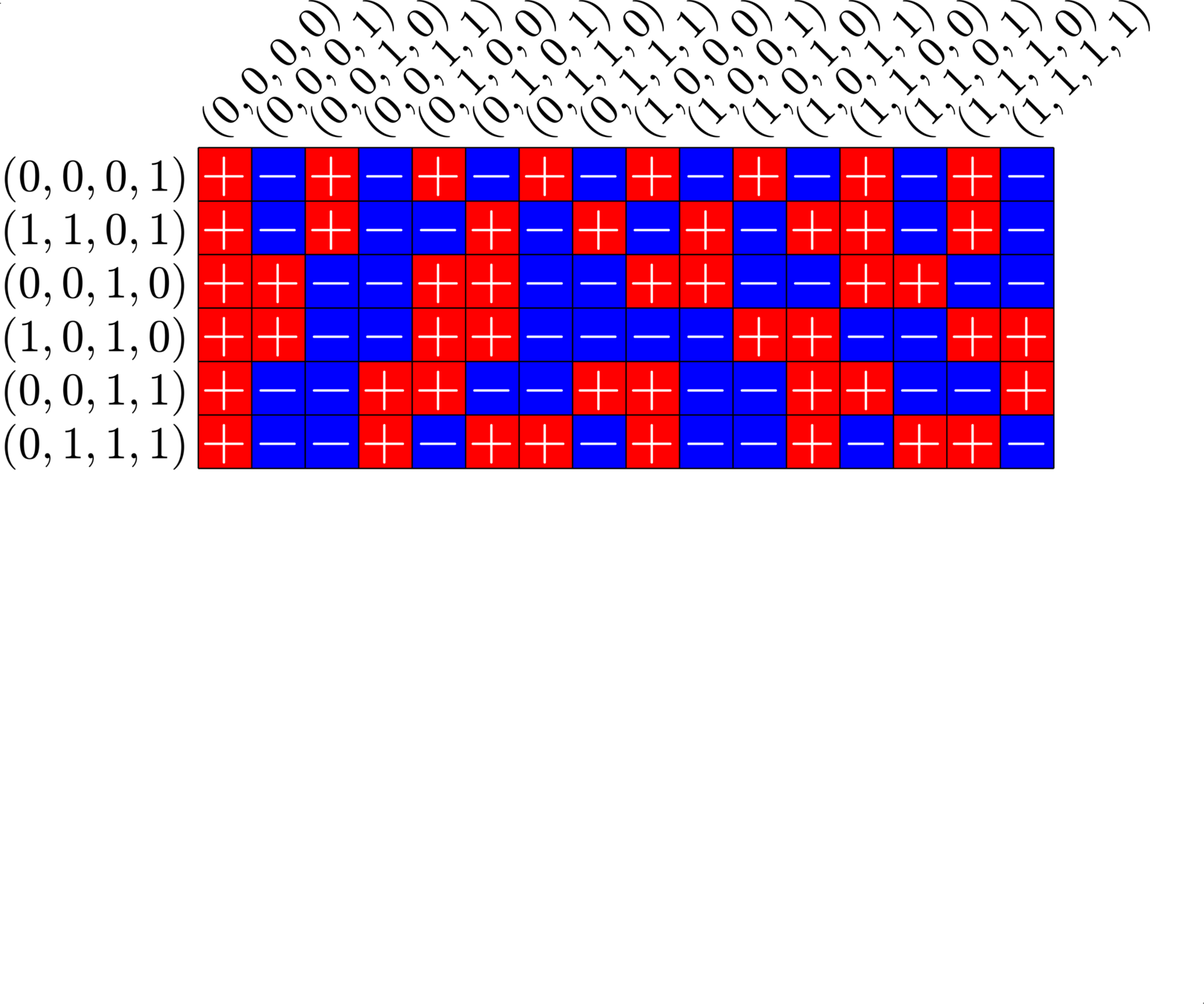
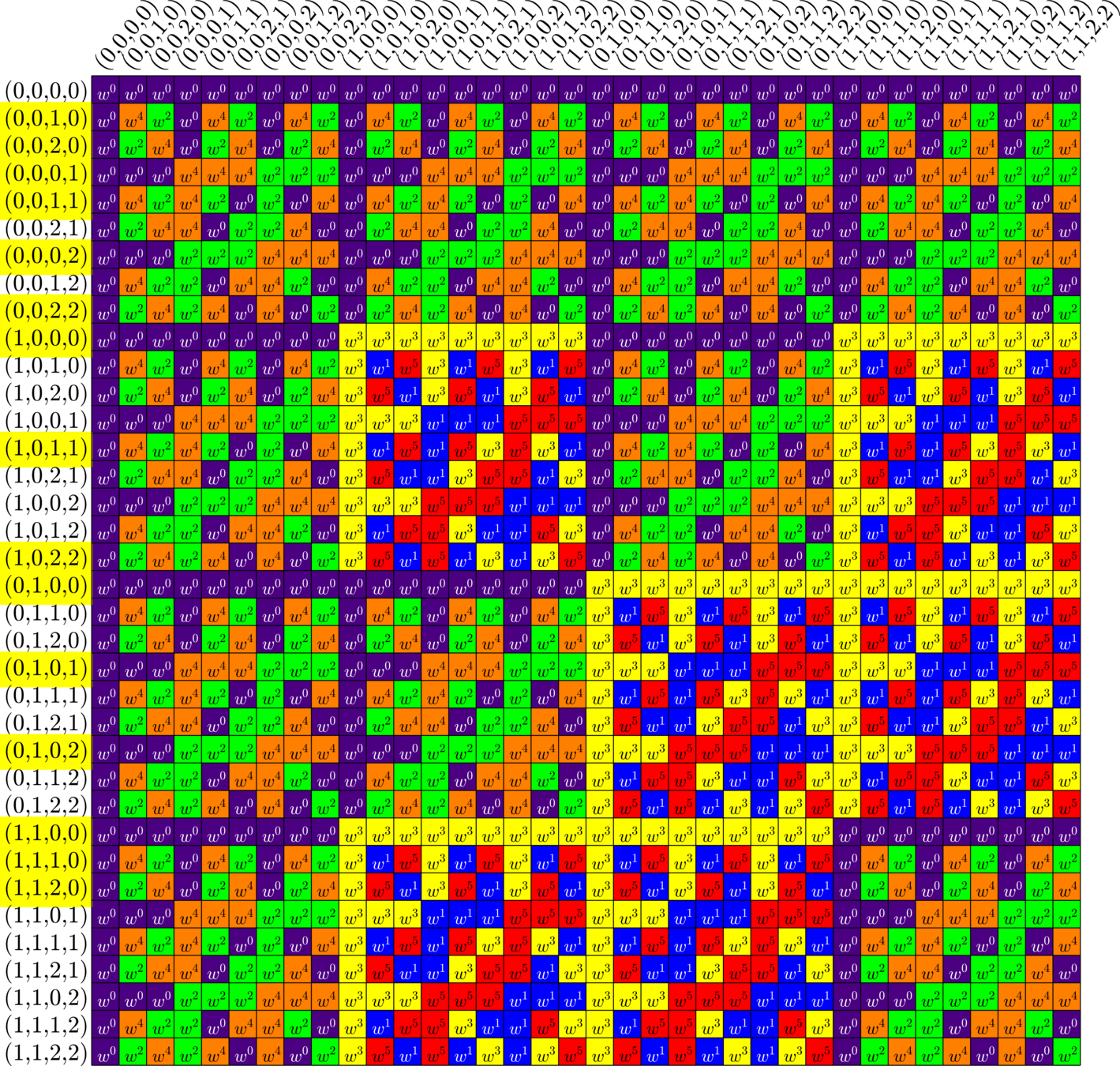
\[\begin{array}{c|cccccc} & (0,0,0,1) & (1,1,0,1) & (0,0,1,0) & (1,0,1,0) & (0,0,1,1) & (0,1,1,1)\\ \hline (0,0,0,1) & (0,0,0,0) & (1,1,0,0) & (0,0,1,1) & (1,0,1,1) & (0,0,1,0) & (0,1,1,0)\\ (1,1,0,1) & (1,1,0,0) & (0,0,0,0) & (1,1,1,1) & (0,1,1,1) & (1,1,1,0) & (1,0,1,0)\\ (0,0,1,0) & (0,0,1,1) & (1,1,1,1) & (0,0,0,0) & (1,0,0,0) & (0,0,0,1) & (0,1,0,1)\\ (1,0,1,0) & (1,0,1,1) & (0,1,1,1) & (1,0,0,0) & (0,0,0,0) & (1,0,0,1) &(1,1,0,1)\\ (0,0,1,1) & (0,0,1,0) & (1,1,1,0) & (0,0,0,1) & (1,0,0,1) & (0,0,0,0) & (0,1,0,0)\\ (0,1,1,1) & (0,1,1,0) & (1,0,1,0) & (0,1,0,1) & (1,1,0,1) & (0,1,0,0) & (0,0,0,0) \end{array}\]
\[D=\{(0,0,0,1),(0,0,1,0),(0,0,1,1),(0,1,1,1),(1,0,1,0),(1,1,0,1)\}\]
is a (McFarland) difference set in \(G=\Z_{2}\times\Z_{2}\times\Z_{2}\times\Z_{2}\)
A McFarland difference set
The subgroup \[H=\Z_{2}\times \Z_{2}\times 0\times 0\leqslant G\] is disjoint from \(D\).
A McFarland difference set

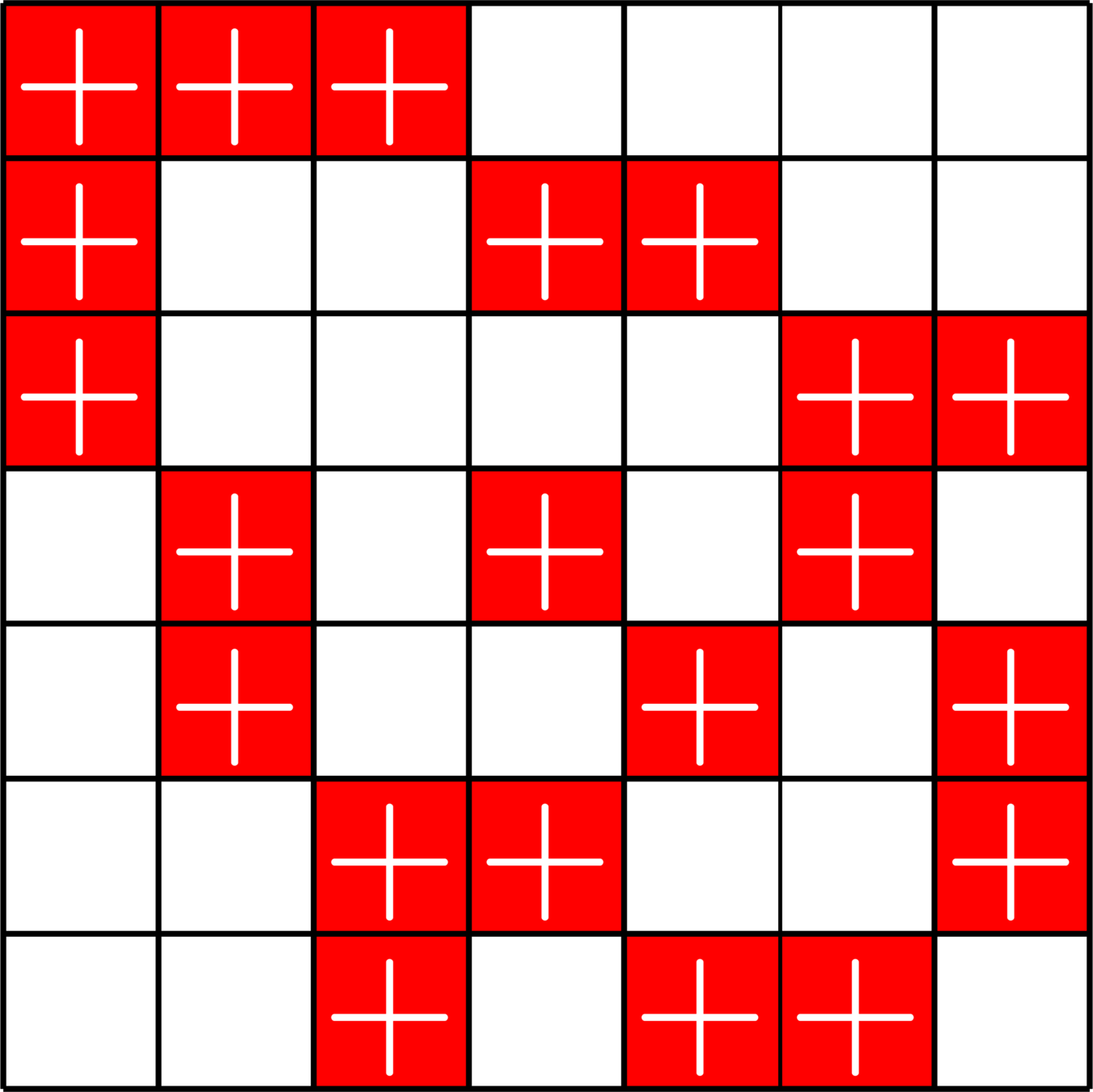
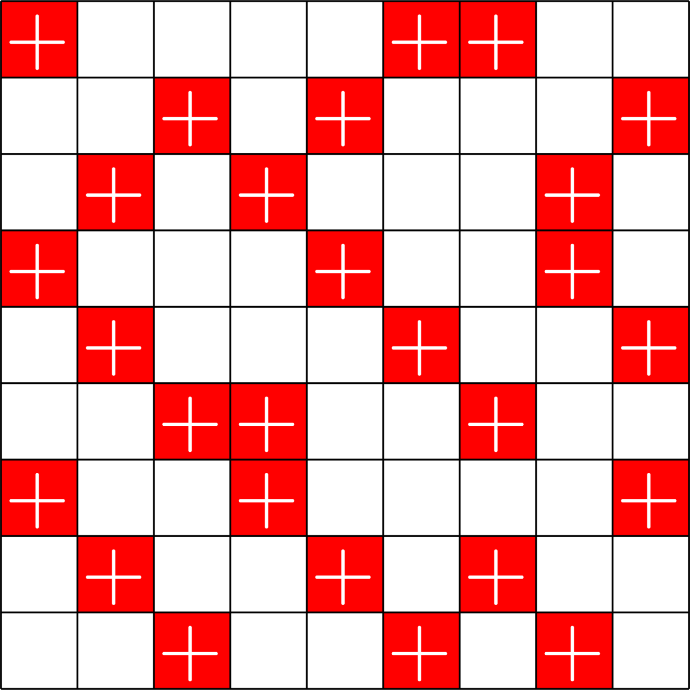
Steiner Systems
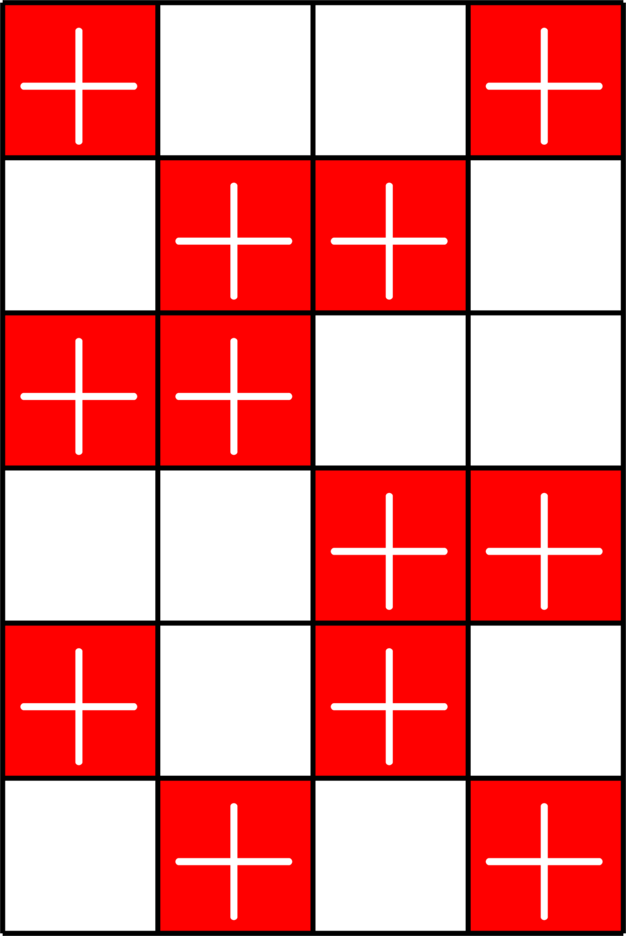
Definition. A \((2,k,v)\)-Steiner system is a \(\{0,1\}\)-matrix \(X\) such that:
- Each row of \(X\) has exactly \(k\) ones.
- Each column of \(X\) has exactly \(r=\frac{v-1}{k-1}\) ones.
- The dot product of any pair of distinct columns is one.
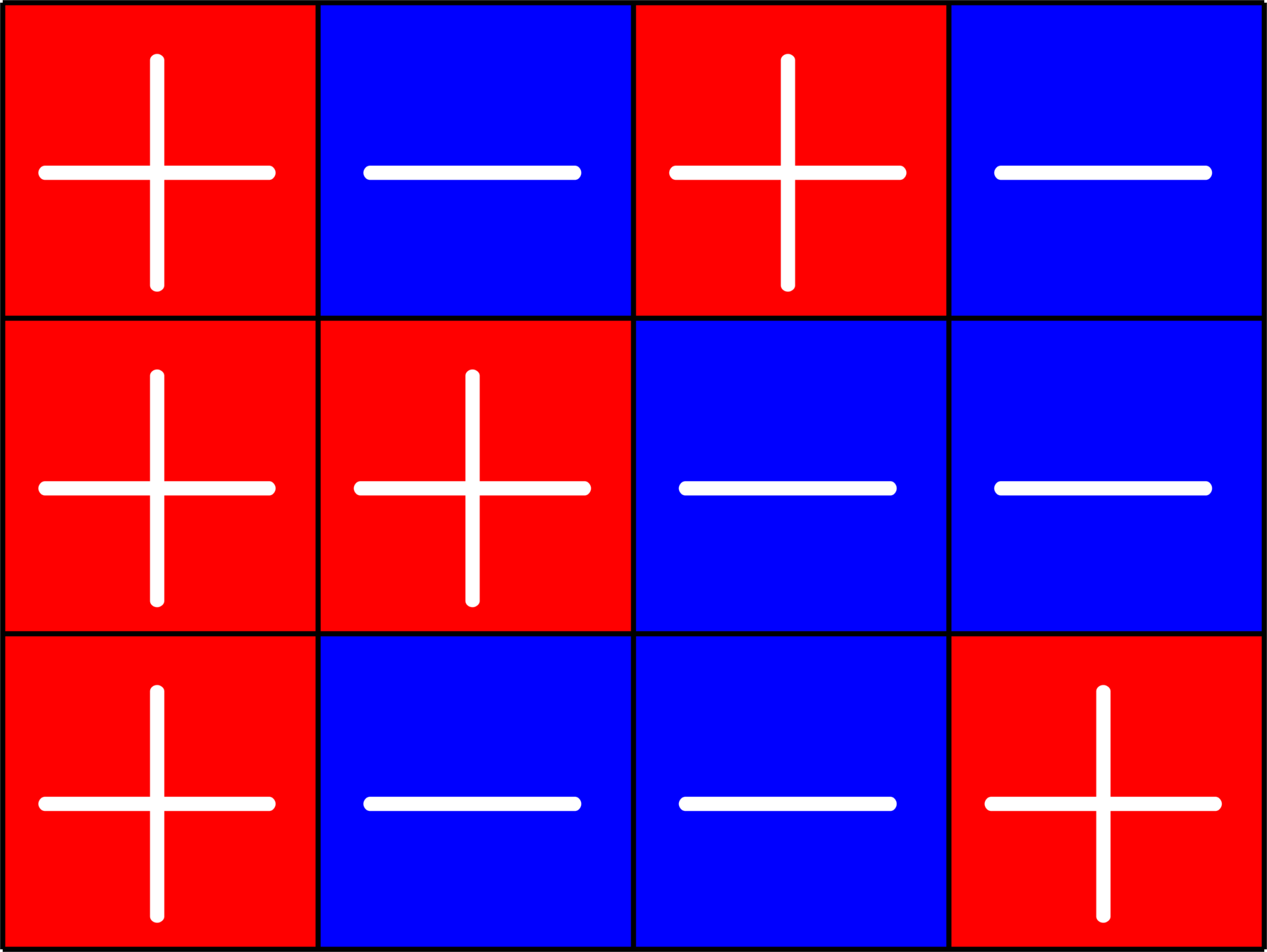
Example. The matrix
\(X = \)
is a \((2,2,4)\)-Steiner system.

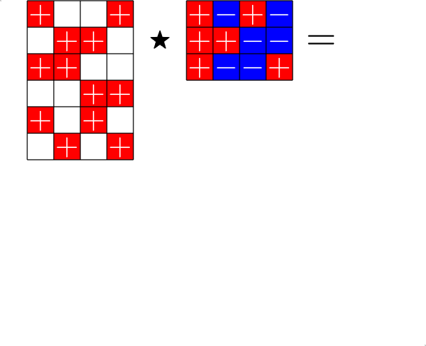
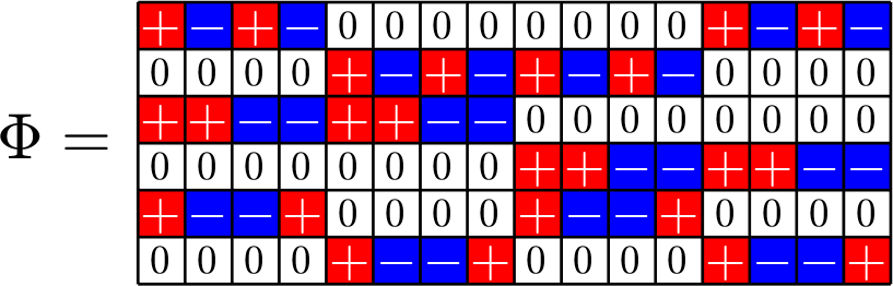
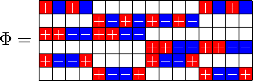
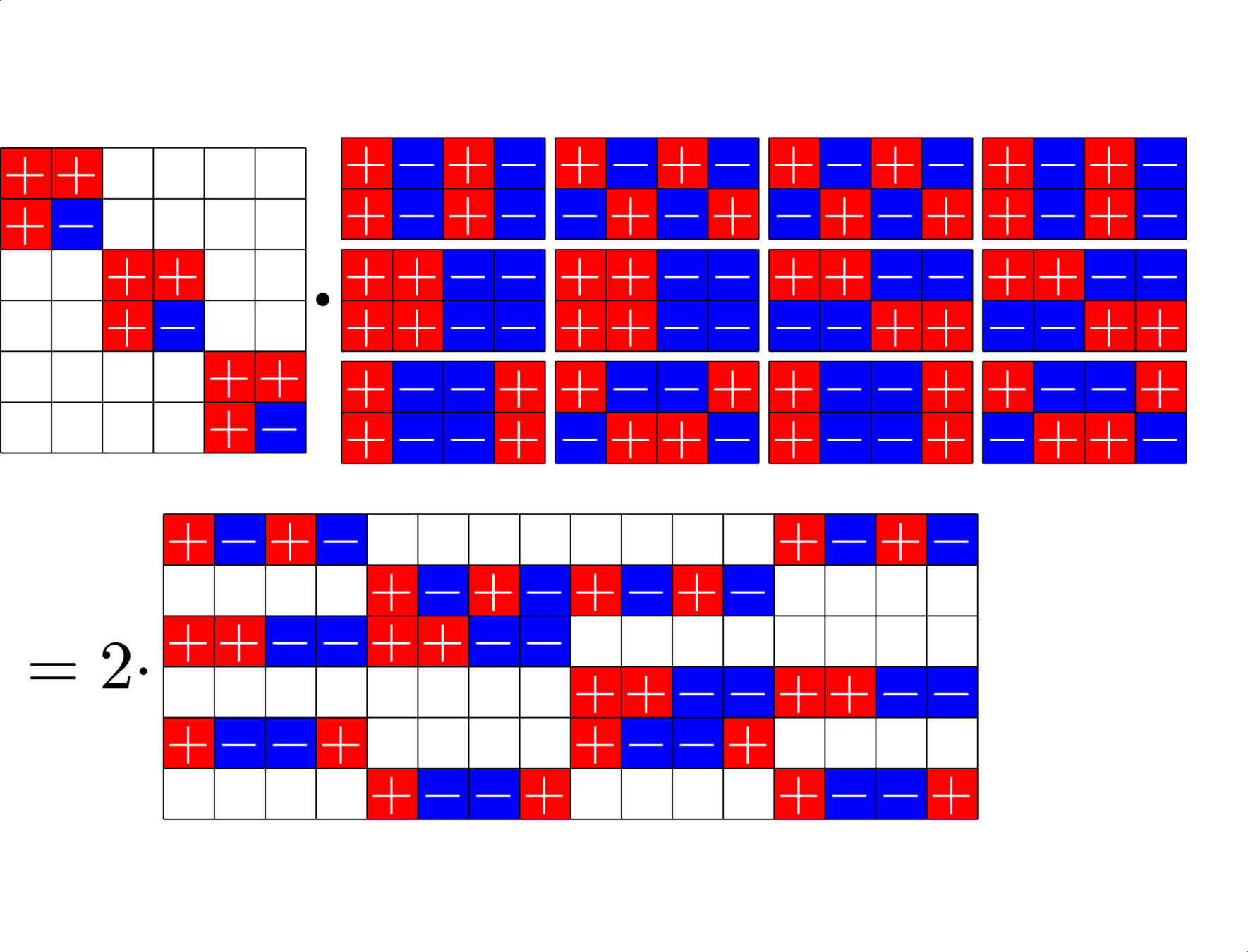
The Star Product
A way to construct lots of ETFs
\(=\)
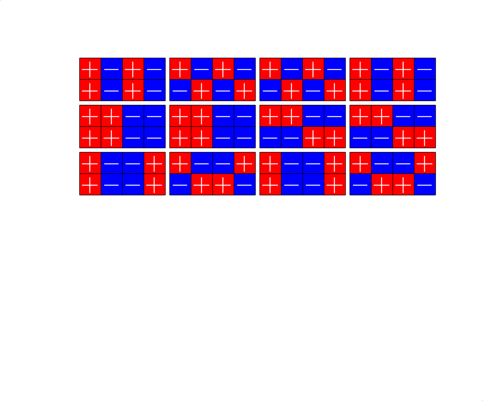
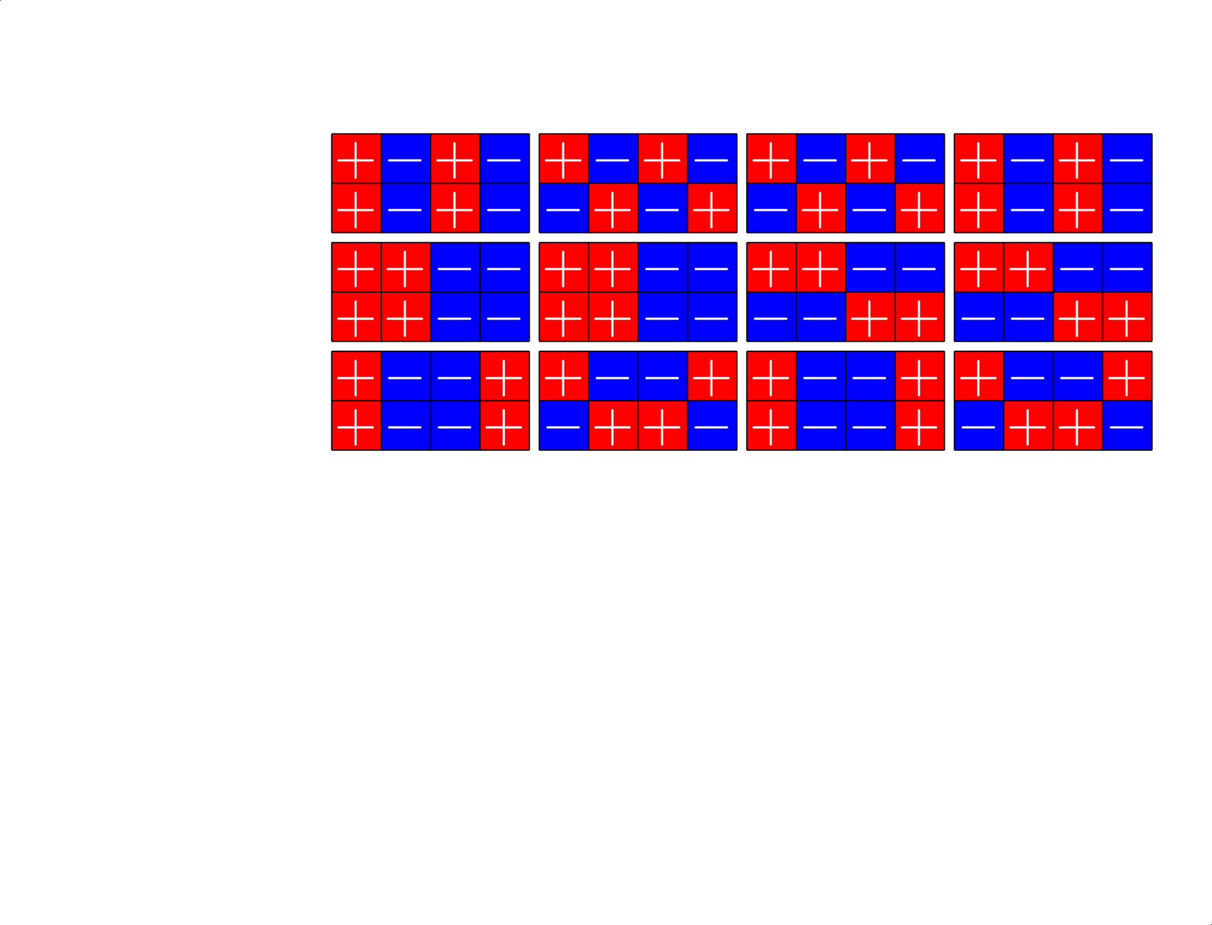
Take a Steiner system with \(r\) ones per column
and an \(r\times (r+1)\) ETF with unimodular entries
The Star product is a "Steiner" ETF
Roadmap for this talk
Vectors that are "Spread out"
Equiangular tight frames
ETFs from groups
\(\Z_{2}\times\Z_{2}\times\Z_{2}\times\Z_{2}\)
The design theory underneath
Real Flat ETFs
Some binary codes
Group divisible designs
ETFs and graphs
Packing points
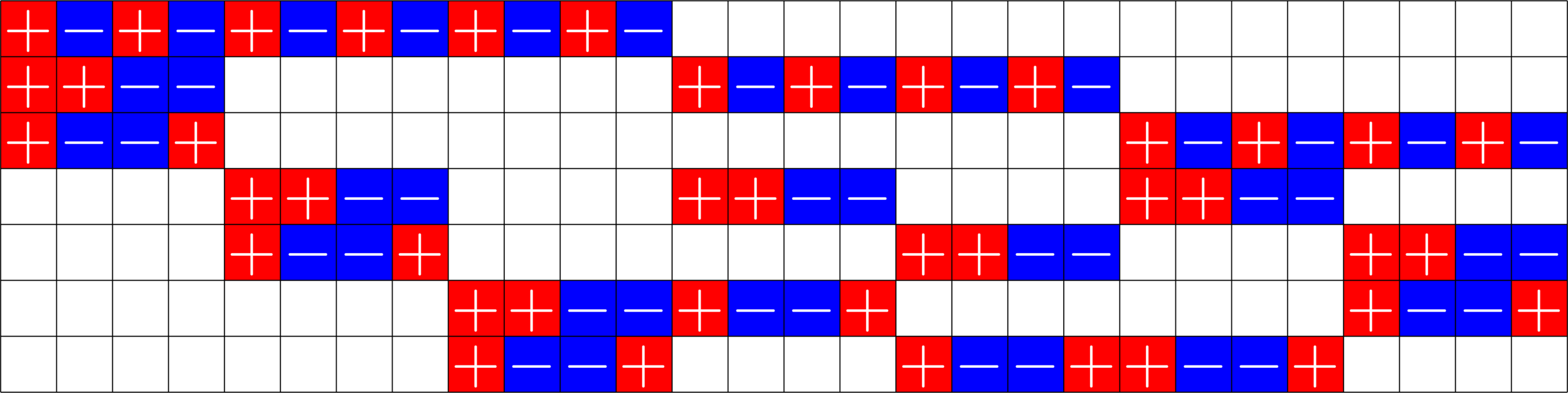
Real Flat ETFs

ETFs with all \(\pm 1\) entries: Real Flat ETFs
Why real flat ETFs?
- Waveform design: maximize \(\|x\|_{2}\) subject to \(\|x\|_{\infty}\leq B\) (minimal peak-to-average power ratio)
- Quasi-symmetric designs
- Grey-Rankin equality binary codes
Real Flat ETFs

Real Flat ETFs

\(=\)
Real Flat ETFs

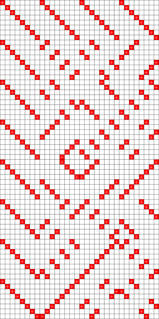
Example. A \(276\times 576\) real ETF

Real Flat ETFs
Theorem (J '13)
\(N\times N\) Hadamard matrix \(\Longrightarrow\) \(N(2N-1)\times 4N^2\) real flat ETF
Previously known real flat ETFs:
- \(N = 2^k\) harmonic ETFs on \(\mathbb{Z}_{2}^{2k+2}\)
- \(N = 6\) [Bracken, McGuire, & Ward, 2006]
Theorem (Mixon, J, Fickus '13)
Real Flat
ETFs
Grey-Rankin
equality
binary codes

1-1 correspondence
We can also construct a real flat \(317886556\times 1907416992\) ETF.
Roadmap for this talk
Vectors that are "Spread out"
Equiangular tight frames
ETFs from groups
\(\Z_{2}\times\Z_{2}\times\Z_{2}\times\Z_{2}\)
The design theory underneath
Real Flat ETFs
Some binary codes
Group divisible designs
ETFs and graphs
Packing points
Meme of the talk:
\(\mathbb{Z}_{2}\times\mathbb{Z}_{2}\times\mathbb{Z}_{3}\times\mathbb{Z}_{3}\)
Some ETFs
arise from
Spence Difference Sets...
a lot more ETFs
arise from
Group Divisible
Designs!
Ex:
\(G\)
\( \mathbb{Z}_{2}\)
\(\times\)
\(\mathbb{Z}_{2}\)
\(\times\)
\(\mathbb{Z}_{3}\)
\(\times\)
\(\mathbb{Z}_{3}\)
\(=\)


\(\bigotimes\)

\[\left[\begin{array}{l} \\ \\ \\ \\ \\ \\ \\ \\ \\ \\ \\ \end{array}\right.\]
\[\left.\begin{array}{l} \\ \\ \\ \\ \\ \\ \\ \\ \\ \\ \\ \end{array}\right]\]

\[\cong\]
Unitary transformation
\(I_{3}\otimes\)(\(2\times 3\) ETF)
\(3\times 4\) ETF with unimodular entries
???
Group Divisible Designs
Definition. A \(K\)-GDD of type \(M^{U}\) is a \(\{0,1\}\)-matrix \(X\) such that:
- \(X\) has \(UM\) columns.
- Each row of \(X\) has \(K\) ones.
- \(X^{\top}X = R\cdot I_{UM}+J_{UM}-(I_{U}\otimes J_{M})\) for some \(R\in\N\)
Example. The following is a \(3\)-GDD of type \(3^3\):
\(X = \)

\(X^{\top}X = \)
ETFs from GDDs
Theorem (Fickus, J '19). Given a
\(d\times n\) ETF
\(k\)-GDD of type \(M^{U}\)
and
provided certain integrality conditions hold, there exists a \(D\times N\) ETF with \(D>d\), \(N>n\) and \(\frac{D}{N}\approx \frac{d}{n}.\)
A New ETF
This GDD
Combined with a \(6\times 16\) ETF, like this one:
produces a complex \(266\times 1008\) ETF, which appears to be new!
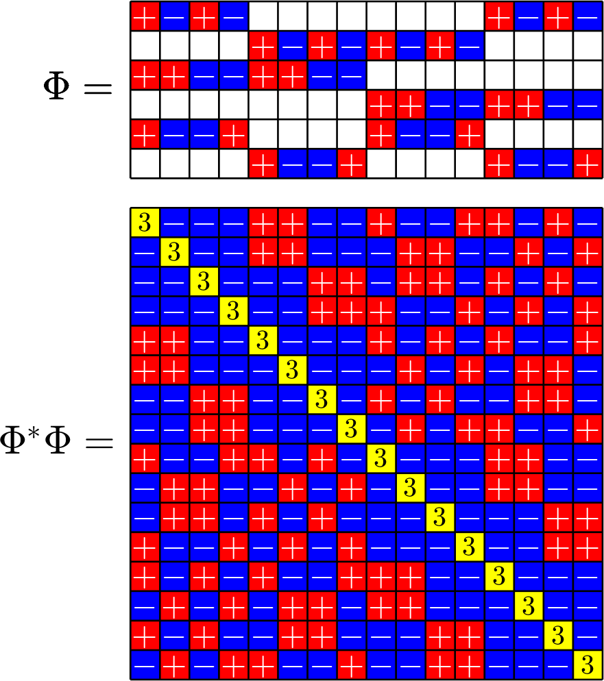
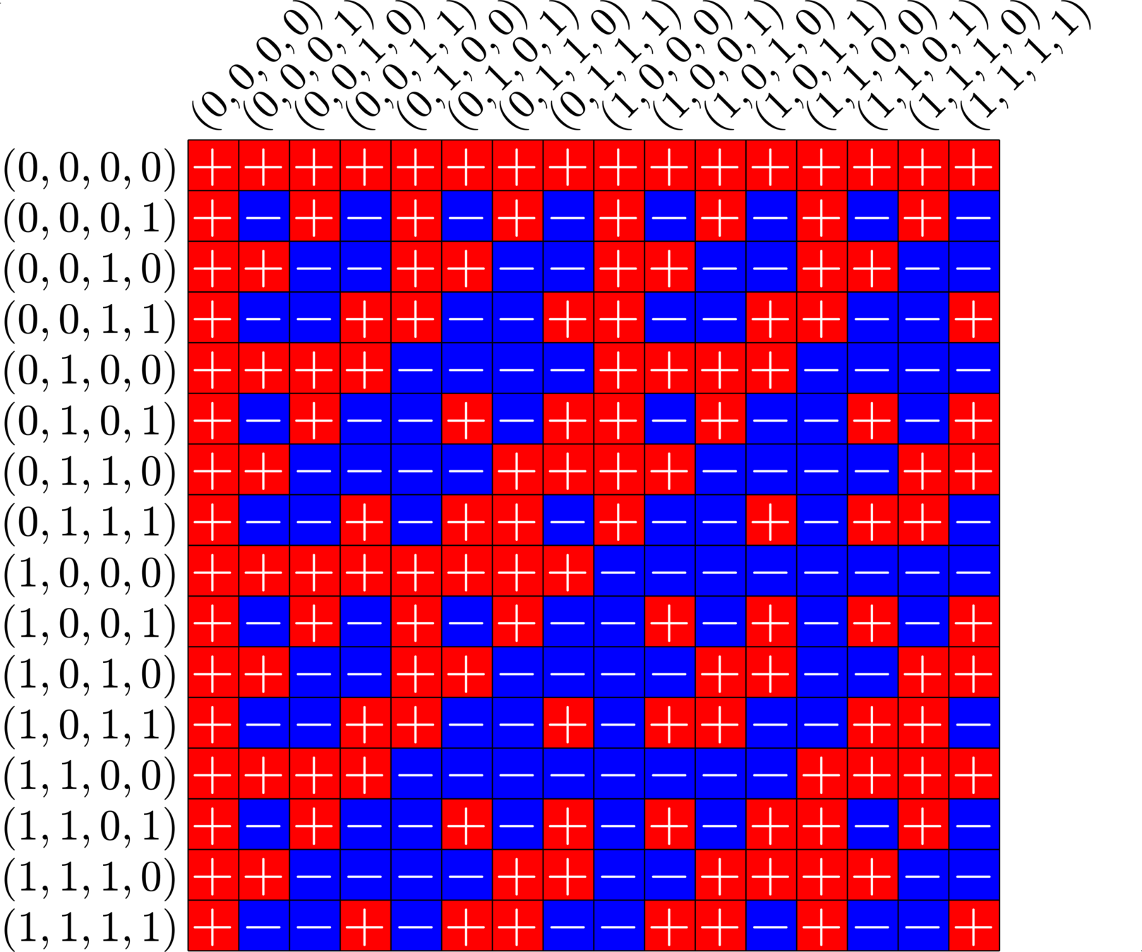
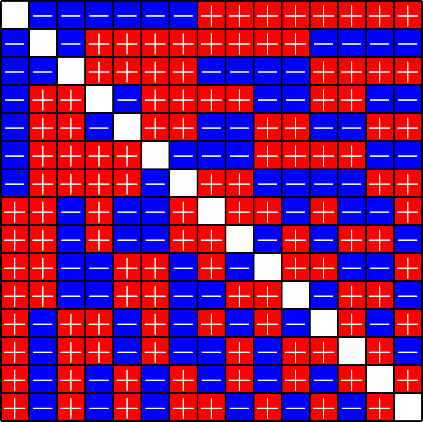
Real ETFs and Graphs
\(\Phi=\)
- Given a real ETF \(\Phi\)
- Normalize so that all dot products with the first vector are positive.
Real ETFs and Graphs
\(\Phi^{\top}\Phi=\)
- Given a real ETF \(\Phi\)
- Normalize so that all dot products with the first vector are positive.
- Look at the gram matrix \(\Phi^{\top}\Phi\)
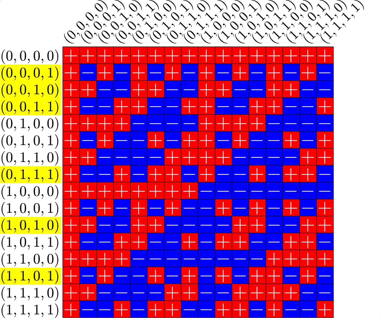
Real ETFs and Graphs
- Given a real ETF \(\Phi\)
- Normalize so that all dot products with the first vector are positive.
- Look at the gram matrix \(\Phi^{\top}\Phi\)
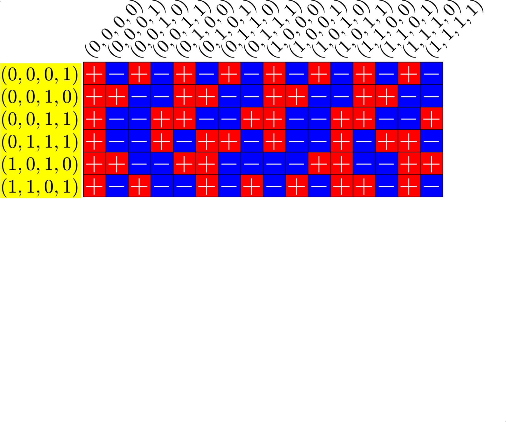
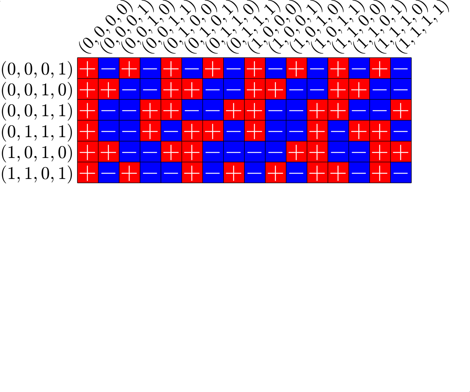
- Remove the first row and column and zero out the diagonal
Real ETFs and Graphs
- Given a real ETF \(\Phi\)
- Normalize so that all dot products with the first vector are positive.
- Look at the gram matrix \(\Phi^{\top}\Phi\)
- Remove the first row and column and zero out the diagonal
- This is the Seidel adjacency matrix of a strongly regular graph

Real ETFs and Graphs
A. E. Brouwer maintains a table of known strongly regular graphs.


Our approach:
Real
ETFs
Combinatorial
designs
Strongly
regular graph
Construct
object
Certify
novelty
Rocky Mountain Algebraic Combinatorics Seminar I
By John Jasper


