New strongly regular graphs from real line packings
John Jasper
Air Force Institute of Technology
Rocky Mountain Algebraic Combinatorics Seminar
The views expressed in this talk are those of the speaker and do not reflect the official policy
or position of the United States Air Force, Department of Defense, or the U.S. Government.
https://slides.com/johnjasper/rmacs2/
special optimizers have nice repn's
nice repn's \(\Rightarrow\) rare graphs
Outline
find vectors maximally "spread out"
Background
Vectors that are as spread out as possible
Theorem (the Welch bound). For unit vectors \(\Phi=(\varphi_{i})_{i=1}^{N}\) in \(\mathbb{R}^d\)
\[\mu(\Phi)\geq \sqrt{\frac{N-d}{d(N-1)}}.\]
Equality holds if and only if both:
- Tight: There is a constant \(A>0\) such that \[\sum_{i=1}^{N}|\langle v,\varphi_{i}\rangle|^{2} = A\|v\|^{2} \quad\text{for all } v.\]
- Equiangular: There is a constant \(\alpha\) such that \[|\langle\varphi_{i},\varphi_{j}\rangle| = \alpha\quad\text{for all }i\neq j.\]
Welch bound equality \(\Longleftrightarrow\) equiangular tight frame (ETF)
ETF Gram matrix
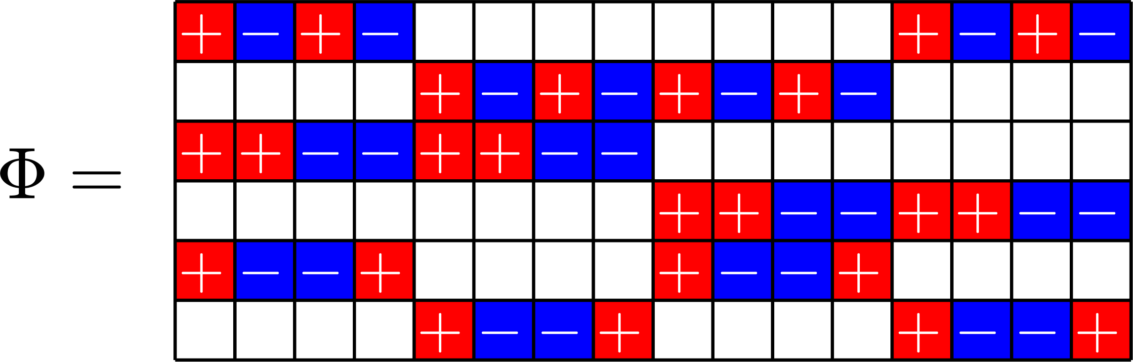
Definition. Let \[\Phi = \big[\varphi_{1}\ \ \varphi_{2}\ \ \cdots\ \ \varphi_{N}\big]\in \mathbb{R}^{d\times N},\]
be a rank \(d\) matrix where each column \(\varphi_{n}\) is unit norm
\[\|\varphi_{n} \|^{2}=1.\]
1) (Tightness) \(\exists\,A>0\) such that \((\Phi^{\top}\Phi)^{2} = A\Phi^{\top}\Phi\).
2) (Equiangular) \(\exists\,B>0\) such that \(|\frac{1}{B}\varphi_{m}^{\top}\varphi_{n}^{}|=1\) for \(m\neq n\).
If both 1) and 2) hold, then \(\{\varphi_{n}\}_{n=1}^{N}\) is an ETF(\(d,N)\).
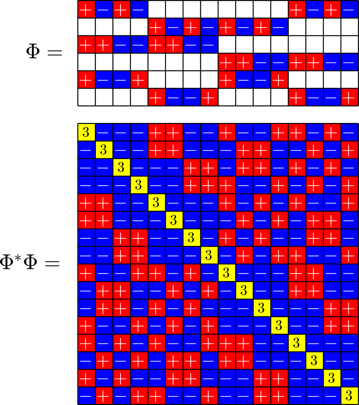
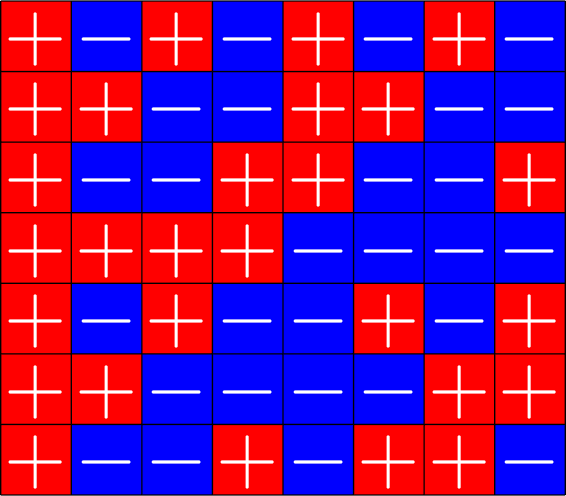
\[\Phi^{\top}\Phi = \left[\begin{array}{cccc} 1 & \varphi_{1}^{\top}\varphi_{2} & \cdots & \varphi_{1}^{\top}\varphi_{N}\\[1ex] \varphi_{2}^{\top}\varphi_{1} & 1 & \cdots & \varphi_{2}^{\top}\varphi_{N}\\[1ex] \vdots & \vdots & \ddots & \vdots\\[1ex] \varphi_{N}^{\top}\varphi_{1} & \varphi_{N}^{\top}\varphi_{2} & \cdots & 1\end{array}\right]\]
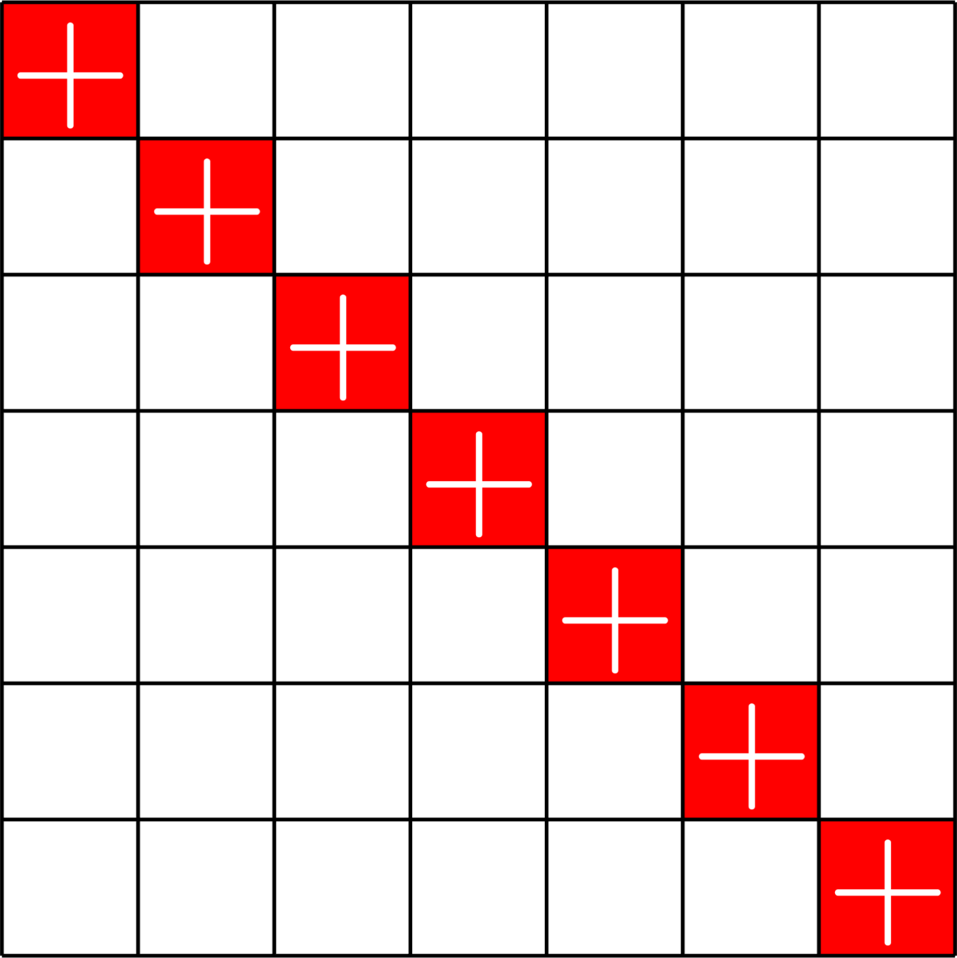
\(1\)'s down the diagonal
1) \(\Phi^{\top}\Phi \propto\) projection
2) \(|\varphi_{m}^{\top}\varphi_{n}^{}|\) constant

\(=\)
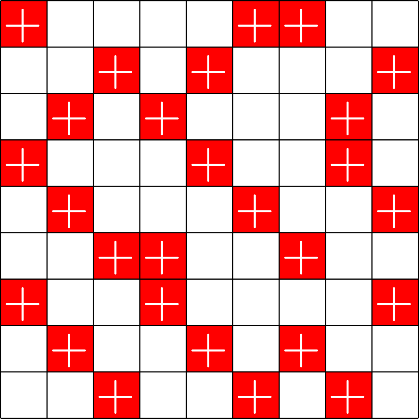
Steiner system
\(r\) ones per column
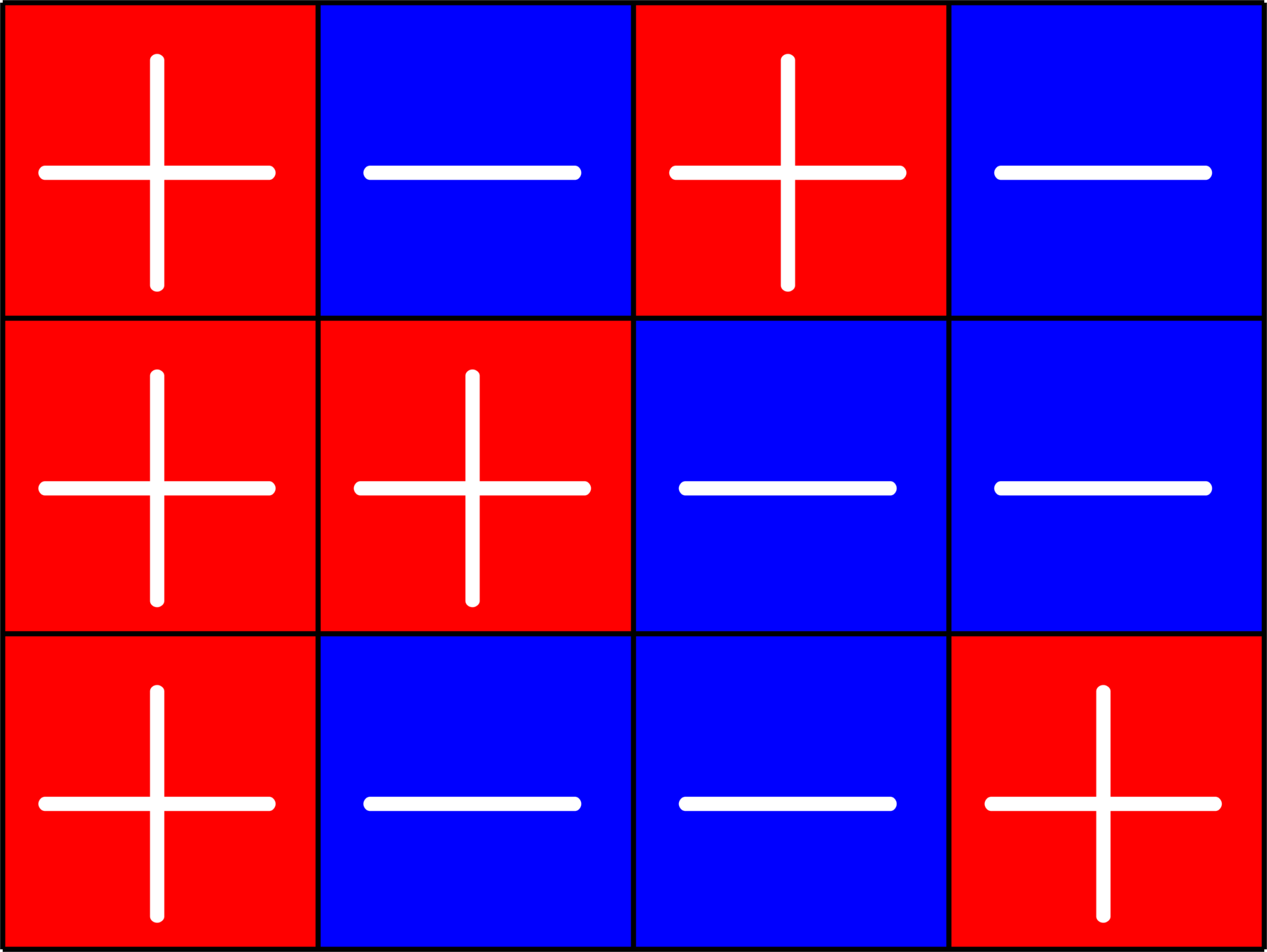
\(r\times (r+1)\) ETF with unimodular entries
"Steiner" ETF
16 vectors in \(\mathbb{R}^{6}\)

It's easy to go this way
\(\Phi^{\top}\Phi=\)
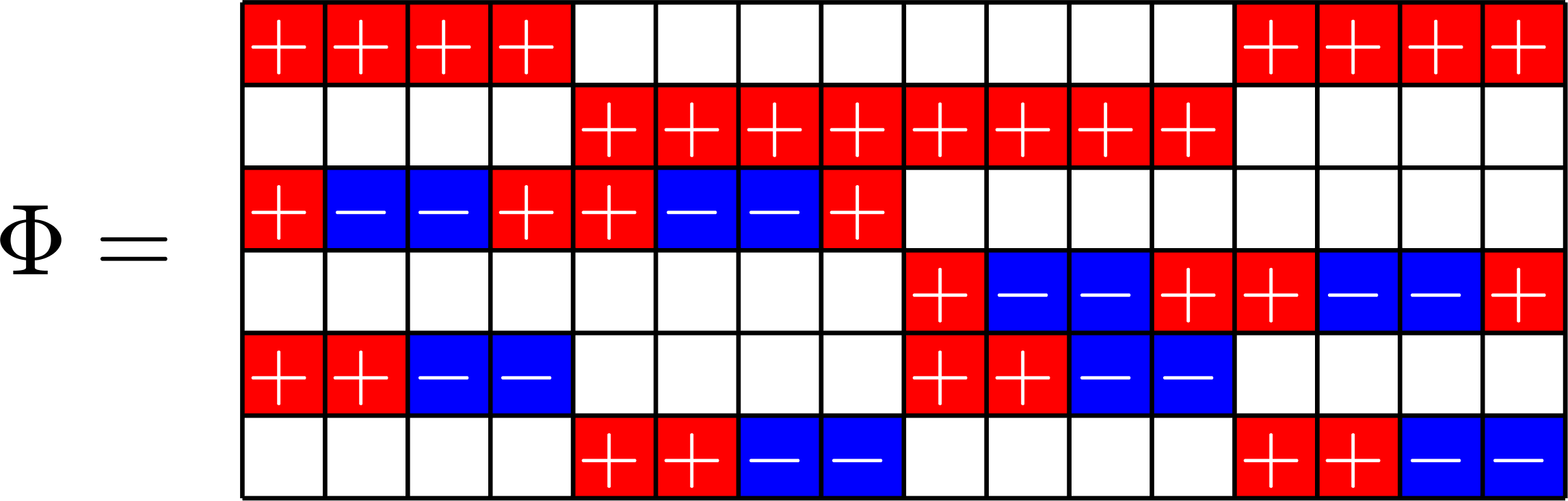
\(\Phi=\)
Gramians are forgetful
Given \(\Phi^{\top}\Phi\),
\(\Phi\) is only determined up to a unitary

\(\Phi^{\top}\Phi=\)
\(\Phi=\)

Gram matrix of ETF:
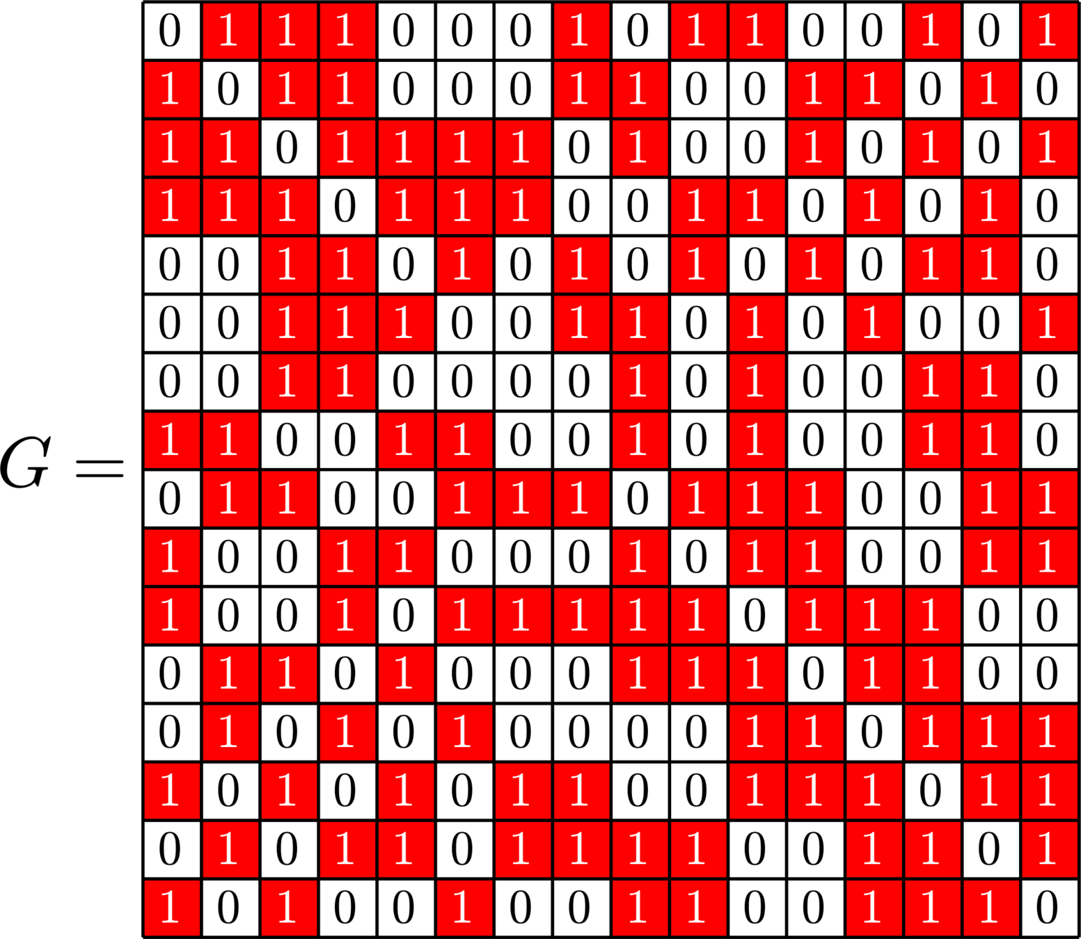
Adjacency matrix of graph:
ETFs \(\Rightarrow\) Graphs
- Every vertex has 9 neighbors
- Adjacent vertices have 4 common neighbors
- Non-adjacent vertices have 6 common neighbors
Replace diagonal 1's with 0's
Replace -1's with 1's
Zero out the diagonal
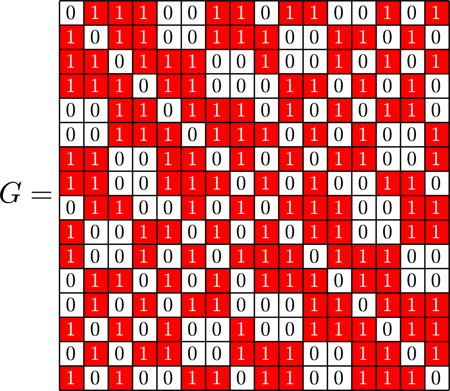

Mult. by \(-1\)
Not regular!
Strongly Regular Graphs
Definition. An \(n\)-vertex graph is called strongly regular if
- every vertex has \(k\) neighbors
- adjacent vertices have \(\lambda\) common neighbors
- nonadjacent vertices have \(\mu\) common neighbors
Such a graph is called an SRG\((n,k,\lambda,\mu)\).
Equivalently, the adjacency matrix \(G\) satisfies
\[G^{2} = k I + \lambda G + \mu(J-I-G)\quad\text{(where \(J\) is the all-ones matrix.)}\]
\(\Phi\) ETF \(\Rightarrow\) "quadratic relation":
\[(\Phi^{\top}\Phi)^{2} = A\,\Phi^{\top}\Phi.\]
But how many \(-1\)'s in each row ???
ETF \(\Rightarrow\) SRG
\(\Rightarrow\) the associated graph is regular and thus strongly regular
\(\mathbf{1}\) is an eigenvector of \(\Phi^{\top}\Phi\).
- \(\mathbf{1} := (1,1,\ldots,1)\in\ker\Phi\)
- \(\mathbf{1}\) \(\in\) row space of \(\Phi\), or
}
\(\Leftrightarrow\)
\(\mathbf{1}\) in row space
SRG\((16,5,0,2)\)
\(\mathbf{1}\in\ker\Phi\)
SRG\((16,9,4,6)\)
Example.
Nice ETF representation \(\Rightarrow\) new SRGs!
Suppose \(\Phi\) is an ETF:
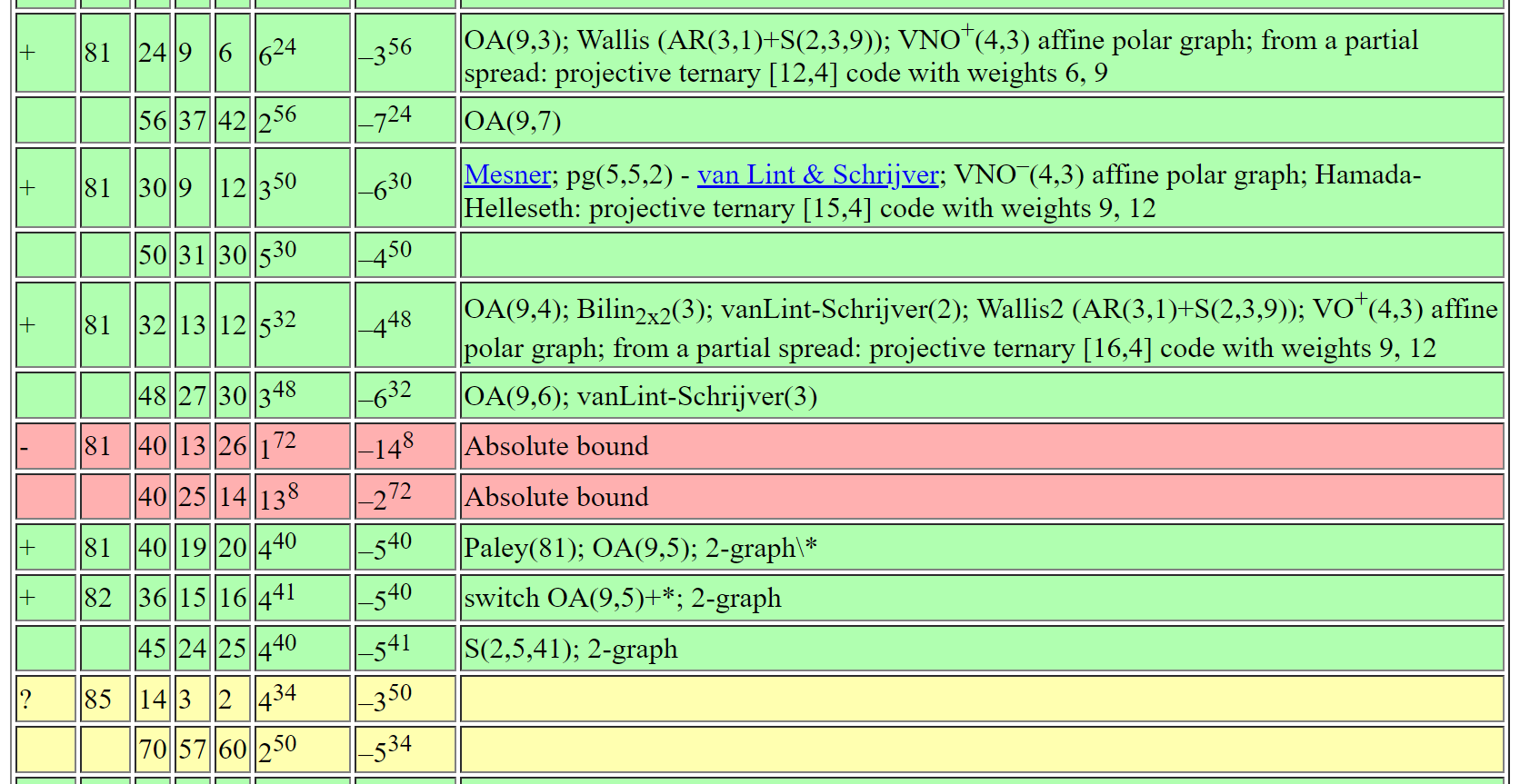

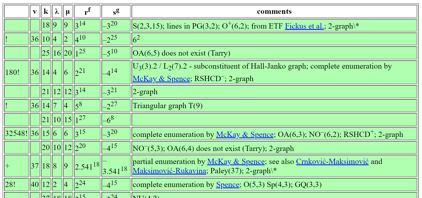
Andries Brouwer's Table of SRGs
= \(\nexists\)
= ???
= \(\exists\)
Goal: \(\mapsto\)
Prototype
Tremain ETFs

\[\left[\begin{array}{l} \\ \\ \\ \\ \\ \\ \\ \\ \\ \\ \\ \\ \\ \\ \\ \\ \\ \end{array}\right.\]
\[\left.\begin{array}{l} \\ \\ \\ \\ \\ \\ \\ \\ \\ \\ \\ \\ \\ \\ \\ \\ \\ \end{array}\right]\]

\(\bigotimes\)
\(\sqrt{2}\)
\(\sqrt{\dfrac{1}{2}}\)
\(\sqrt{\dfrac{3}{2}}\)

Hadamard matrix
Hadamard matrix
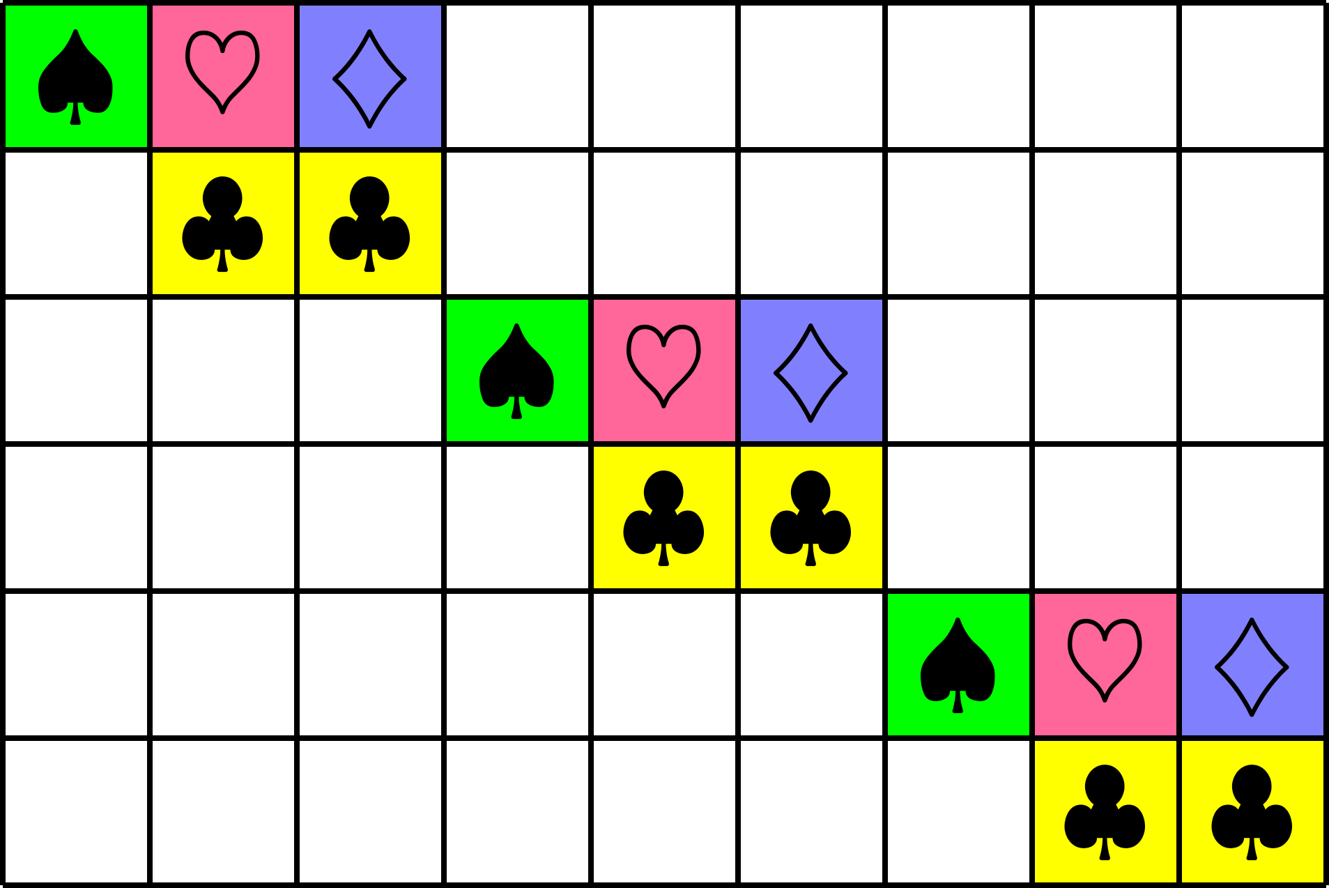
Steiner Triple System
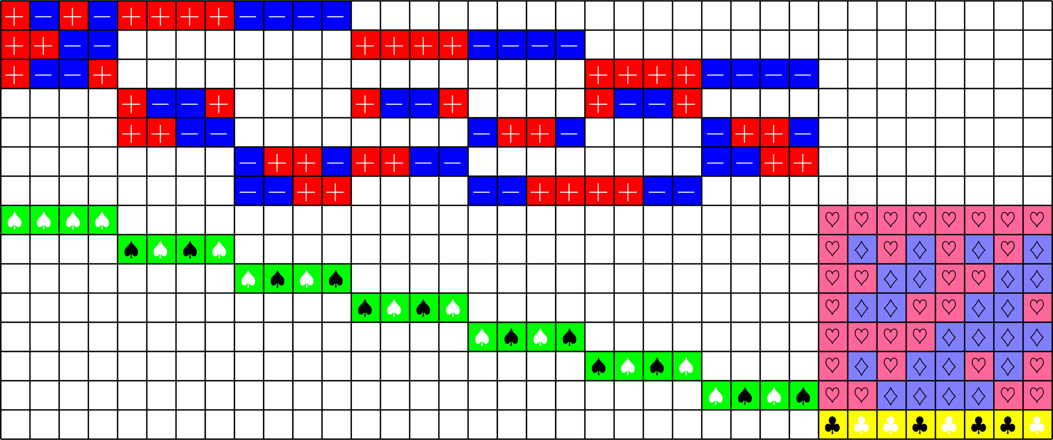
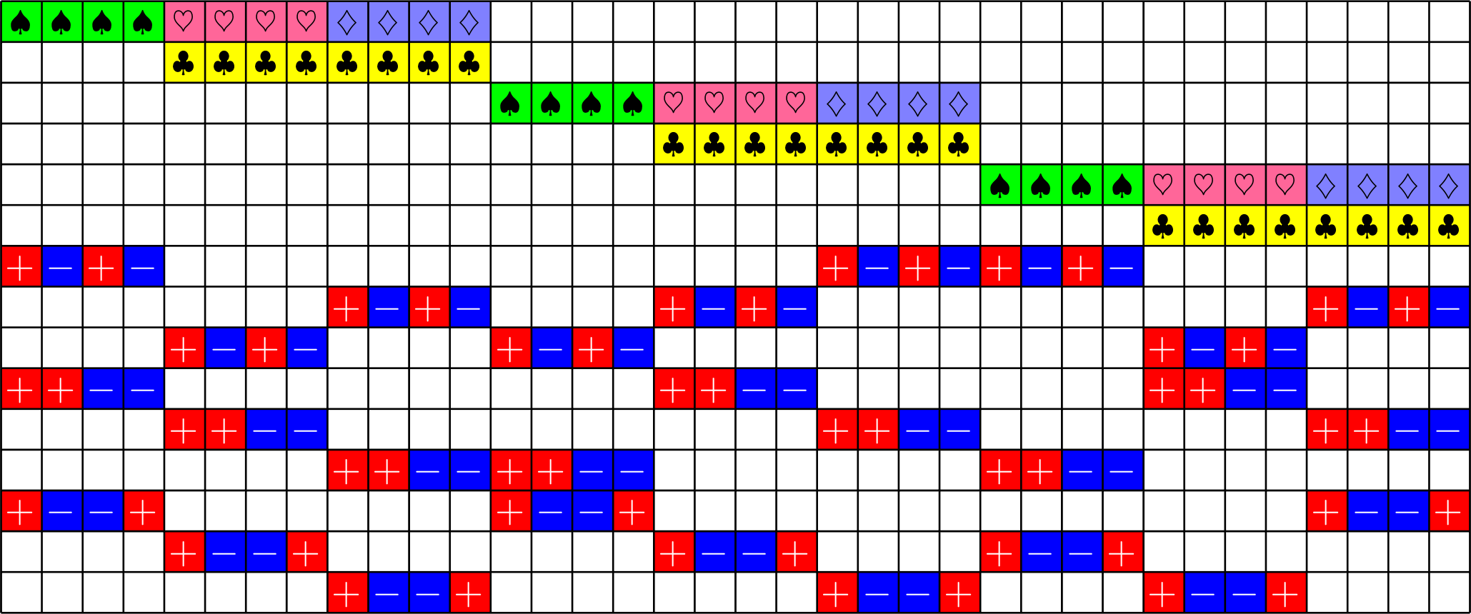
Tremain ETFs


\(\ =+1\)
\(\ =-1\)
\(\ =\sqrt{2}\)
\(\ =-\sqrt{\dfrac{1}{2}}\)
\(\ =+\sqrt{\dfrac{1}{2}}\)
\(\ =\sqrt{\dfrac{3}{2}}\)
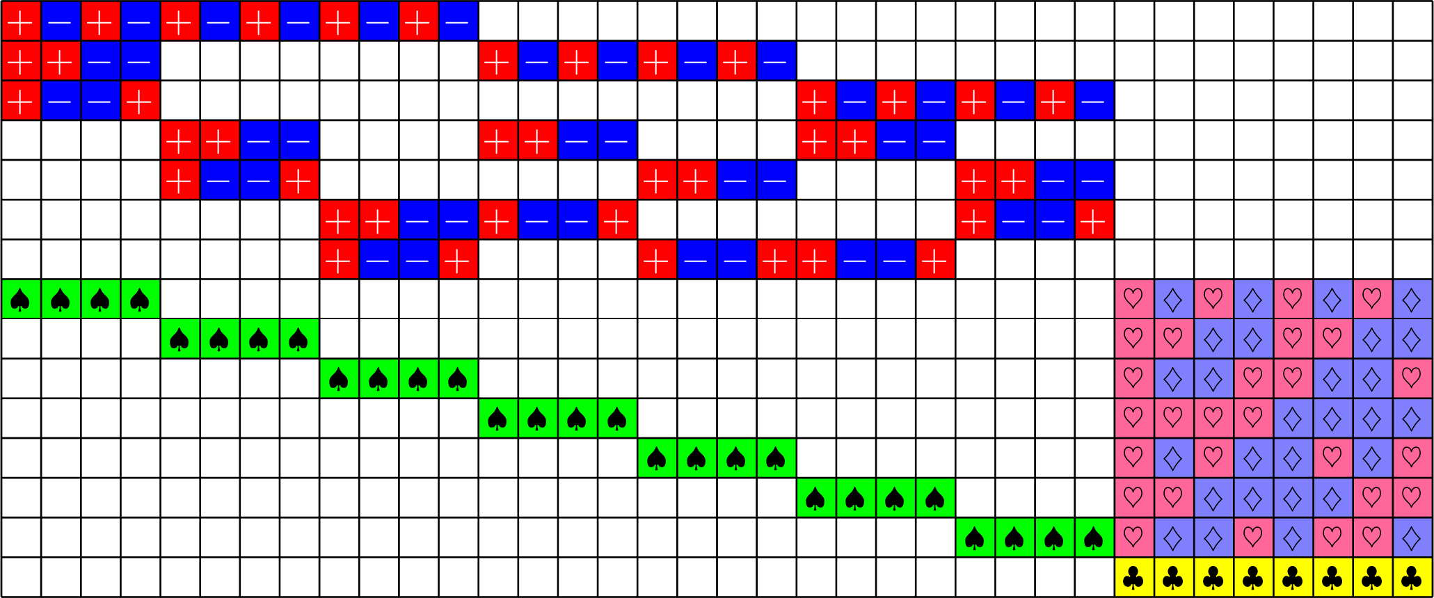
Tremain ETFs:
Theorem (Fickus, J, Mixon, Peterson '18). If there exists an
\(h\times h\) Hadamard matrix with \(h\equiv 1\) or \(2\) \(\text{mod}\ 3\),
then there exists a \((2,3,2h-1)\)-Steiner system
and by the Tremain construction there exists a real \(d\times N\) ETF where \[d=\frac{1}{3}(h+1)(2h+1),\qquad N=h(2h+1).\]
\(51\times 136\) Tremain ETF
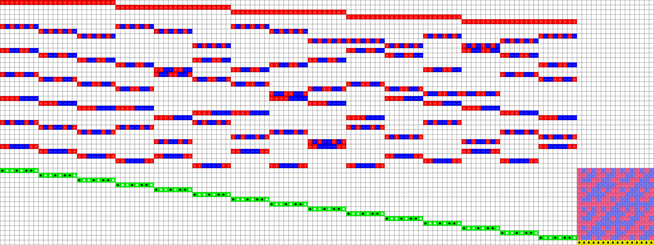
\(\ =+1\)
\(\ =-1\)
\(\ =\sqrt{2}\)
\(\ =-\sqrt{\dfrac{1}{2}}\)
\(\ =+\sqrt{\dfrac{1}{2}}\)
\(\ =\sqrt{\dfrac{3}{2}}\)


\(\ =-\sqrt{2}\)
\(\ =-\sqrt{\dfrac{3}{2}}\)
Axial Tremain ETFs:
Theorem (Fickus, J, Mixon, Peterson '18). If there exists an
\(h\times h\) Hadamard matrix with \(h\equiv 2\) \(\text{mod}\ 3\),
then there exists a strongly regular graph with parameters:
\[v=h(2h+1),\ k=\frac{(h+2)(2h-1)}{2},\ \lambda=\frac{(h-1)(h+4)}{2},\ \mu = \frac{h(h+2)}{2}\]
This gave us a new ETF!
From Brouwer's table online:
Let's replicate this success!
New Results
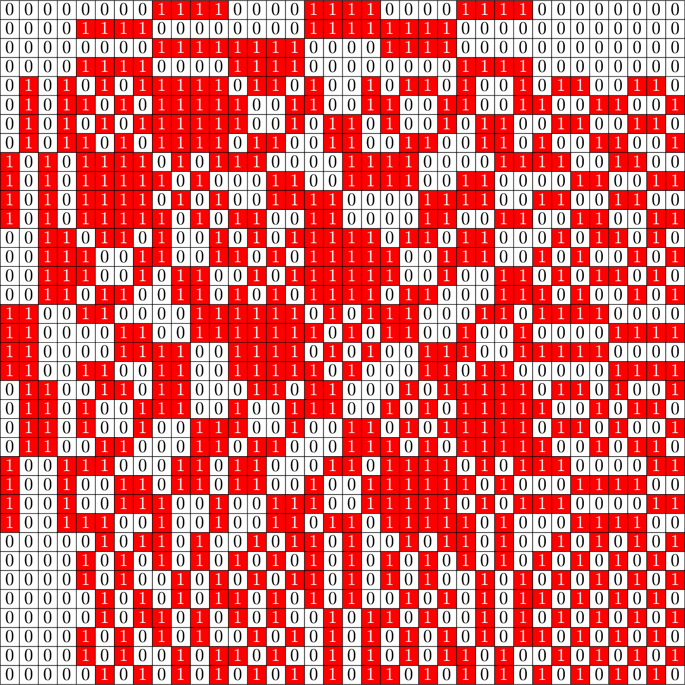
How can I make these vectors sum to zero?
\(\ =+1\)
\(\ =-1\)
\(\ =\sqrt{2}\)
\(\ =-\sqrt{\dfrac{1}{2}}\)
\(\ =+\sqrt{\dfrac{1}{2}}\)
\(\ =\sqrt{\dfrac{3}{2}}\)
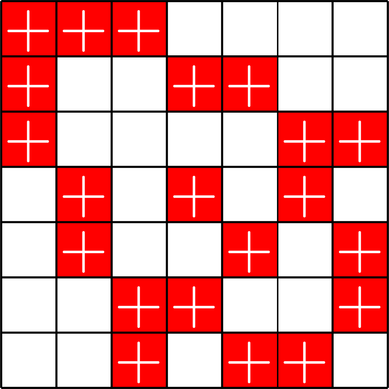
Graph from a \(15\times 36\) ETF with \(\boldsymbol{1}\) the kernel
Back to Brouwer's Table
\(\operatorname{NO}^{-}\)(6,2)
Nice short fat repn ?

\(NO_{6}^{-}(2)\)

\(\Phi^{\top}\Phi=\)
\(\Phi=\)
Remember: Gramians are forgetful

\(NO_{6}^{-}(2)\)


\(NO_{6}^{-}(2)\)
\(\ =+1\)
\(\ =-1\)
\(\ =\sqrt{2}\)
\(\ =-\sqrt{\dfrac{1}{2}}\)
\(\ =+\sqrt{\dfrac{1}{2}}\)
\(\ =\sqrt{\dfrac{3}{2}}\)
\(\ =-\sqrt{2}\)
\(\ =-\sqrt{\dfrac{3}{2}}\)
\(NO_{6}^{-}(2)\)
- \(\mathbf{1} = (1,1,\ldots,1)\) is in the kernel
- works for all real Tremain ETFs!
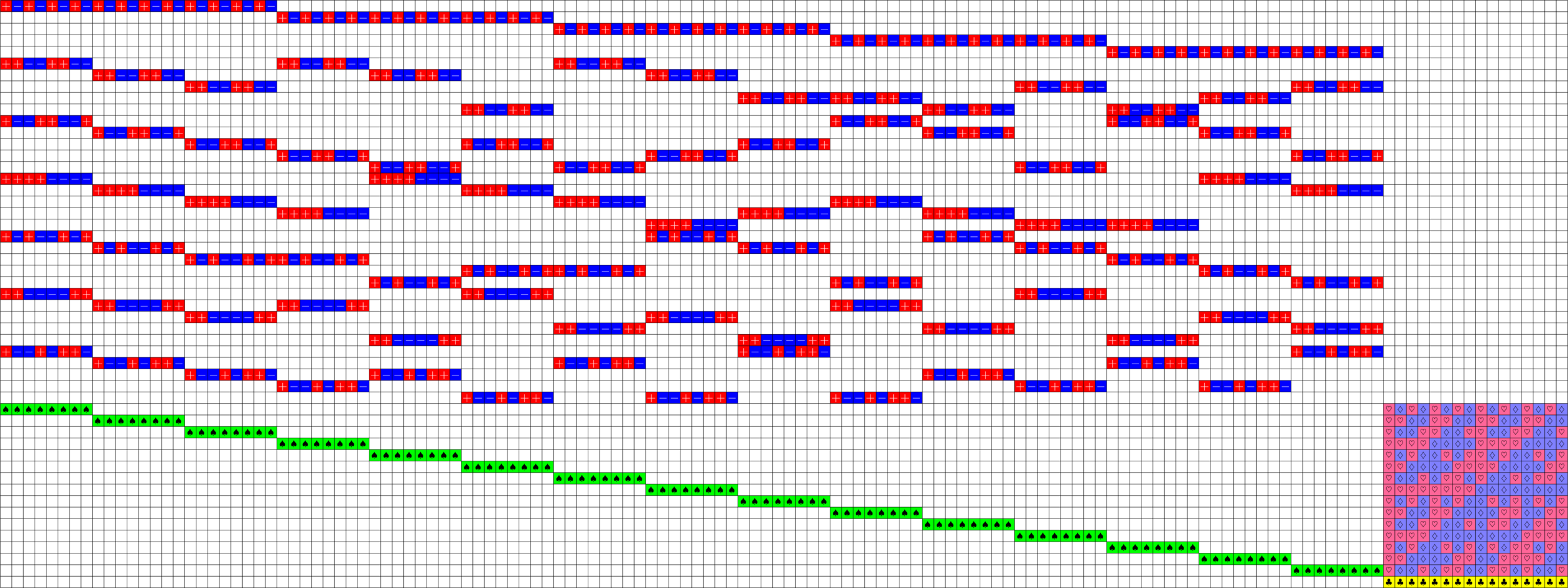
Centered Tremain ETFs:
Theorem (J). If there exists an
\(h\times h\) Hadamard matrix with \(h\equiv 1\) or \(2\) \(\text{mod}\ 3\),
then there exists a strongly regular graph with parameters
\[v=h(2h+1),\quad k=h^2-1,\quad \lambda=\frac{1}{2}(h^2-4),\quad \mu = \frac{1}{2}h(h-1)\]
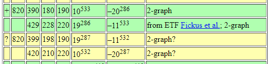
\(\exists\, 20\times 20\) Hadamard matrix \(\Rightarrow\) SRG(820,399,198,190)
From Brouwer's table online:

\(\exists\, 20\times 20\) Hadamard matrix \(\Rightarrow\) SRG(820,399,198,190)
\(\bigotimes\)

\[\left[\begin{array}{l} \\ \\ \\ \\ \\ \\ \\ \\ \\ \\ \\ \end{array}\right.\]
\[\left.\begin{array}{l} \\ \\ \\ \\ \\ \\ \\ \\ \\ \\ \\ \end{array}\right]\]
\(I_{3}\otimes\)(\(2\times 3\) ETF)
Hadamard Matrix
Group Divisible Design (GDD)
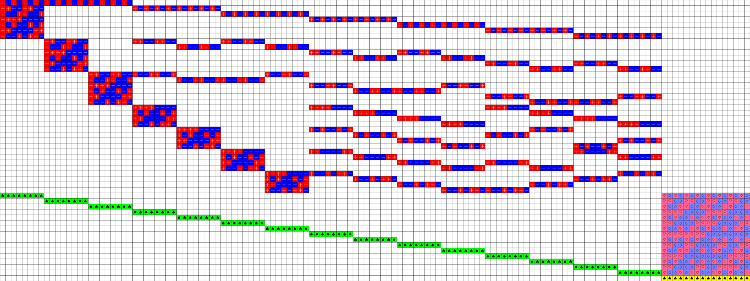
Group Divisible Design
\(\ =+1\)
\(\ =-1\)
\(\ =\sqrt{2}\)
\(\ =-\sqrt{\dfrac{1}{2}}\)
\(\ =+\sqrt{\dfrac{1}{2}}\)
\(\ =\sqrt{\dfrac{3}{2}}\)
\(\ =-\sqrt{2}\)
\(\ =-\sqrt{\dfrac{3}{2}}\)
Group Divisible Design
\(\ =+1\)
\(\ =-1\)
\(\ =\sqrt{2}\)
\(\ =-\sqrt{\dfrac{1}{2}}\)
\(\ =+\sqrt{\dfrac{1}{2}}\)
\(\ =\sqrt{\dfrac{3}{2}}\)
\(\ =-\sqrt{2}\)
\(\ =-\sqrt{\dfrac{3}{2}}\)
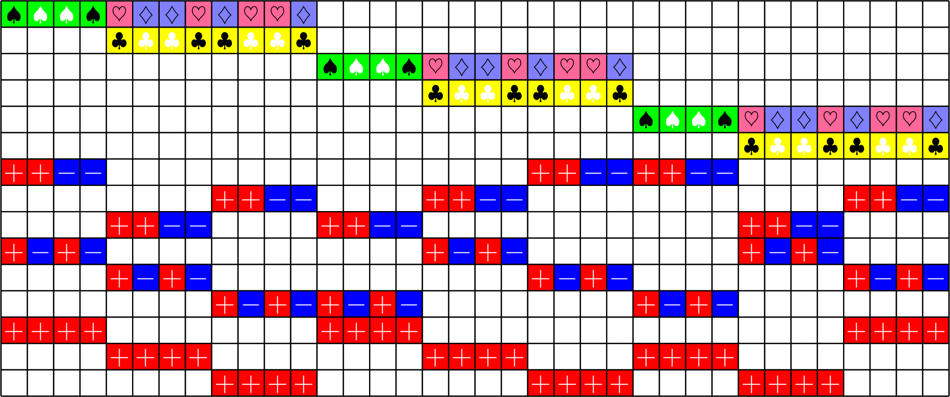
Axial GDD ETFs:
Theorem (J). If there exists an
\(h\times h\) Hadamard matrix with \(h\equiv 1\) \(\text{mod}\ 3\),
then there exists a strongly regular graph with parameters
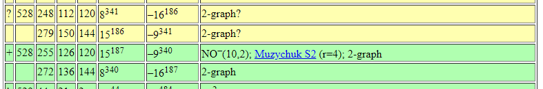
\(\exists\,16\times 16\) Hadamard matrix \(\Rightarrow\exists\) SRG(528,279,150,144)
From Brouwer's table online:
\[v=h(2h+1),\ \ k=\frac{(h+2)(2h-1)}{2},\ \lambda=\frac{(h-1)(h+4)}{2},\ \mu = \frac{h(h+2)}{2}\]
\(\exists\,16\times 16\) Hadamard matrix \(\Rightarrow\exists\) SRG(528,279,150,144)
Compatible Orthobiangular
Tight Frames
Ex:
\(G\)
\( \mathbb{Z}_{2}\)
\(\times\)
\(\mathbb{Z}_{2}\)
\(\times\)
\(\mathbb{Z}_{3}\)
\(\times\)
\(\mathbb{Z}_{3}\)
\(=\)


\(\bigotimes\)
\(\bigotimes\)
\(\bigotimes\)
\(\bigotimes\)
\((0,0)\)
\((0,0)\)
\((1,0)\)
\((0,1)\)
\((1,1)\)
\((1,0)\)
\((0,1)\)
\((1,1)\)


\(\Phi_{0} = \)
\(\Phi_{1} = \)
\(\Phi_{2} = \)
\(\Phi_{3} = \)
\(\Phi_{0}^{\ast}\Phi_{0} = \frac{1}{3}\)


\(\Phi_{1}^{\ast}\Phi_{1} = \frac{1}{3}\)
\(\Phi_{2}^{\ast}\Phi_{2} = \frac{1}{3}\)
\(\Phi_{3}^{\ast}\Phi_{3} = \frac{1}{3}\)


\(+\)
\(+\)
\(+\)
\(=\)
Theorem (Fickus, J, Myers '24). A sequence of matrices with \(M\) columns each
\[\Phi_{0},\Phi_{1},\ldots,\Phi_{L-1}\]
is a compatible orthobiangular tight frame (COBTF) if:
- \(\Phi_{j}^{}\Phi_{j}^{\ast} = A\mathbf{I} (\text{tight, same }A)\)
- Off-diagonal \(\Phi_{j}^{\ast}\Phi_{j}^{}\) has modulus in \(\{0,1\}\) (orthobiangular)
- Off-diagonals supports \(\Phi_{j}^{\ast}\Phi_{j}^{}\) partition
- "Compatibility condition"
If \((h_{i})_{i=0}^{L-1}\) are the rows of a (possibly complex) Hadamard matrix, then
\[\Psi = \begin{bmatrix}\Phi_{0}\otimes h_{0}\\ \Phi_{0}\otimes h_{1}\\ \vdots\\ \Phi_{L-1}\otimes h_{L-1}\end{bmatrix}\]
is an ETF.
COBTF Example 1 (Resolvable Steiner)

\(\Phi_{0}=\)
\[[\]
\[]\]

\(\otimes\)
Parallel classes from resolvable Steiner system
\(\underbrace{\hspace{1in}}\)
\(I_{3}\otimes\)(\(2\times 3\) ETF)
Parallel classes
Group Divisible Design (GDD)
COBTF Example II (Group Divisible Design)
\(\ =+1\)
\(\ =-1\)
\(\ =\sqrt{2}\)
\(\ =-\sqrt{\dfrac{1}{2}}\)
\(\ =+\sqrt{\dfrac{1}{2}}\)
\(\ =\sqrt{\dfrac{3}{2}}\)
\(\ =-\sqrt{2}\)
\(\ =-\sqrt{\dfrac{3}{2}}\)

\(\underbrace{\hspace{1in}}\)
\(\Phi_{0}=\)
\(\Phi_{1}=\)
\(\Phi_{2}=\)
\(\Phi_{3}=\)
\(\otimes\)
\[\left[\begin{array}{l} \\ \\ \\ \\ \\ \\ \\ \\ \\ \\ \\ \end{array}\right.\]
\[\left.\begin{array}{l} \\ \\ \\ \\ \\ \\ \\ \\ \\ \\ \\\\ \end{array}\right]\]
COBTF Example II (Group Divisible Design)
\(\ =+1\)
\(\ =-1\)
\(\ =\sqrt{2}\)
\(\ =-\sqrt{\dfrac{1}{2}}\)
\(\ =+\sqrt{\dfrac{1}{2}}\)
\(\ =\sqrt{\dfrac{3}{2}}\)
\(\ =-\sqrt{2}\)
\(\ =-\sqrt{\dfrac{3}{2}}\)
\(\ =+1\)
\(\ =-1\)
\(\ =\sqrt{2}\)
\(\ =-\sqrt{\dfrac{1}{2}}\)
\(\ =+\sqrt{\dfrac{1}{2}}\)
\(\ =\sqrt{\dfrac{3}{2}}\)
\(\ =-\sqrt{2}\)
\(\ =-\sqrt{\dfrac{3}{2}}\)
COBTF Example II (Group Divisible Design)
Chen's Construction
- Y. Q. Chen (1997): New difference sets!
- Used special sets \(U_{0},\ldots,U_{L-1}\) from a group \(G\)
- \(\Phi_{j}\) by pulling rows \(U_{j}\) from the DFT over \(G\)
- \(\Phi_{0}\) by pulling rows \(G\setminus U_{0}\).
\(U_{0} = \{(0,0),(1,2),(2,1)\}\)
\(U_{1} = \{(0,0),(0,2),(0,1)\}\)
\(U_{2} = \{(0,0),(1,1),(2,2)\}\)
\(U_{3} = \{(0,0),(0,2),(0,1)\}\)
\(\Phi_{0}=\)
\(\Phi_{1}=\)
\(\Phi_{2}=\)
\(\Phi_{3}=\)
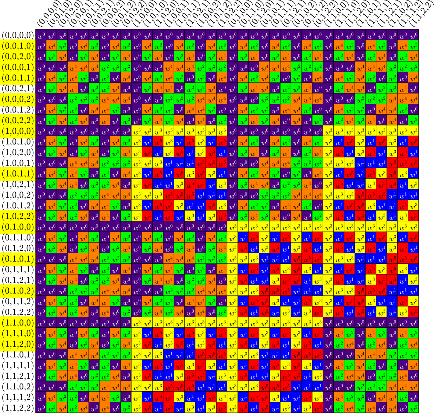
Chen's Construction
- \((\Phi_{j})_{j=0}^{L-1}\) is a COBTF with real gram matrix
- \(L\equiv 0\) (mod \(4\))
- \(L\times L\) Hadamard exists \(\Rightarrow\) new real ETF
- \(\mathbf{1}\) eigenvector of the Gram matrix
- Three new infinite families of SRGs
Example. Chen constructs
\[U_{0},U_{1},\ldots,U_{323}\subset \Z_{3}^{8}\]
This gives us a COBTF \((\Phi_{j})_{j=0}^{323}\).
\(\exists\ 324\times 324\) real Hadamard matrix.
\(\exists\) real \(957177\times 2152008\) ETF.
\(\exists\) SRGs with \(2152007\),
\(2152008\), and \(2152008\) vertices.
Off the charts!

Finding an axial \(77\times 210\)
- Let \(\Phi\) be the known centered \(77\times210\).
- We want to find \(x = \operatorname{argmin}_{\|x\|_{2} = 1}\|\Phi^{\top}x\|_{\infty}\)
- Instead we find \(x = \operatorname{argmin}_{\|x\|_{2} = 1}\|\Phi^{\top}x\|_{4}\)
- Gradient descent on many seeds
- \(\Phi^{\top}x\) is \(\pm1\) vector \(\Rightarrow\) Profit!
There exists an SRG(210,95,40,45)
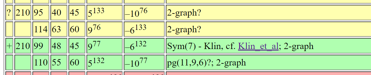
From Brouwer's table online:
There exists an SRG(210,95,40,45)
Thanks!
- This work was partially supported by NSF #1830066
- Webpage: https://tinyurl.com/jasperAFIT
- Slides: https://slides.com/johnjasper

\(\Phi_{0} = \)
\(\Phi_{1} = \)
\(\Phi_{2} = \)
\(\Phi_{3} = \)
Rocky Mountain Algebraic Combinatorics Seminar
By John Jasper


