Day 32:
Least squares and polynomials
Definition. Given an \(m\times n\) matrix \(A\) with singular value decomposition \[A=U\Sigma V^{\top},\] that is, \(U\) and \(V\) are orthogonal matrices, and \(\Sigma\) is an \(m\times n\) diagonal matrix with nonnegative entries \(\sigma_{1}\geq \sigma_{2}\geq \cdots\geq \sigma_{p}\) on the diagonal, we define the pseudoinverse of \(A\) \[A^{+} = V\Sigma^{+}U^{\top}\] where \(\Sigma^{+}\) is the \(n\times m\) diagonal matrix with \(i\)th diagonal entry \(1/\sigma_{i}\) if \(\sigma_{i}\neq 0\) and \(0\) if \(\sigma_{i}=0\).
Example. Consider \[A = \begin{bmatrix} 2 & 0 & 0 & 0\\ 0 & 1 & 0 & 0\\ 0 & 0 & 0 & 0\end{bmatrix}, \quad\text{then}\quad A^{+} = \begin{bmatrix} 1/2 & 0 & 0\\ 0 & 1 & 0\\ 0 & 0 & 0 \\ 0 & 0 & 0 \end{bmatrix}.\]
Example. Consider \[A = \begin{bmatrix} 1 & 0 & 0 & 0\\ 0 & 2 & 0 & 0\\ 0 & 0 & 0 & 0\end{bmatrix}.\]
Then the singular value decomposition of \(A\) is
\[= \begin{bmatrix} 1 & 0 & 0\\ 0 & 1/2 & 0\\ 0 & 0 & 0\\ 0 & 0 & 0\end{bmatrix}.\]
\[A= \begin{bmatrix} 0 & 1 & 0\\ 1 & 0 & 0\\ 0 & 0 & 1\end{bmatrix}\begin{bmatrix} 2 & 0 & 0 & 0\\ 0 & 1 & 0 & 0\\ 0 & 0 & 0 & 0\end{bmatrix}\begin{bmatrix} 0 & 1 & 0 & 0\\ 1 & 0 & 0 & 0\\ 0 & 0 & 1 & 0\\ 0 & 0 & 0 & 1\end{bmatrix}.\]
Hence, the pseudo inverse of \(A\) is
\[A^{+}= \begin{bmatrix} 0 & 1 & 0 & 0\\ 1 & 0 & 0 & 0\\ 0 & 0 & 1 & 0\\ 0 & 0 & 0 & 1\end{bmatrix}\begin{bmatrix} 1/2 & 0 & 0\\ 0 & 1 & 0\\ 0 & 0 & 0\\ 0 & 0 & 0\end{bmatrix}\begin{bmatrix} 0 & 1 & 0\\ 1 & 0 & 0\\ 0 & 0 & 1\end{bmatrix}.\]
Example. Consider \[A = \begin{bmatrix} 1 & 1\\ 1 & 1\end{bmatrix}.\]
Then the singular value decomposition of \(A\) is
\[= \begin{bmatrix}1/4 & 1/4\\ 1/4 & 1/4\end{bmatrix}.\]
\[A= \left(\frac{1}{\sqrt{2}}\begin{bmatrix} 1 & 1\\ 1 & -1\end{bmatrix}\right)\begin{bmatrix} 2 & 0 \\ 0 & 0\end{bmatrix}\left(\frac{1}{\sqrt{2}}\begin{bmatrix} 1 & 1\\ 1 & -1\end{bmatrix}\right).\]
Hence, the pseudo inverse of \(A\) is
\[A^{+}= \left(\frac{1}{\sqrt{2}}\begin{bmatrix} 1 & 1\\ 1 & -1\end{bmatrix}\right)\begin{bmatrix} 1/2 & 0 \\ 0 & 0\end{bmatrix}\left(\frac{1}{\sqrt{2}}\begin{bmatrix} 1 & 1\\ 1 & -1\end{bmatrix}\right).\]
Example. Consider \[B = \begin{bmatrix} 1 & 0 & 1\\ 0 & 1 & 1\end{bmatrix} = \begin{bmatrix} \frac{1}{\sqrt{2}} & \frac{1}{\sqrt{2}}\\[1ex] \frac{1}{\sqrt{2}} & -\frac{1}{\sqrt{2}}\end{bmatrix}\begin{bmatrix} \sqrt{3} & 0 & 0\\ 0 & 1 & 0\end{bmatrix}\begin{bmatrix} \frac{1}{\sqrt{6}} & \frac{1}{\sqrt{6}} & \frac{2}{\sqrt{6}}\\[1ex] \frac{1}{\sqrt{2}} & -\frac{1}{\sqrt{2}} & 0\\[1ex] \frac{1}{\sqrt{3}} & \frac{1}{\sqrt{3}} & -\frac{1}{\sqrt{3}}\end{bmatrix}.\]
Hence, the pseudo inverse of \(B\) is
\[B^{+}=\begin{bmatrix} \frac{1}{\sqrt{6}} & \frac{1}{\sqrt{2}} & \frac{1}{\sqrt{3}}\\[1ex] \frac{1}{\sqrt{6}} & -\frac{1}{\sqrt{2}} & \frac{1}{\sqrt{3}}\\[1ex] \frac{2}{\sqrt{6}} & 0 & -\frac{1}{\sqrt{3}}\end{bmatrix}\begin{bmatrix} 1/\sqrt{3} & 0\\ 0 & 1\\ 0 & 0\end{bmatrix}\begin{bmatrix} \frac{1}{\sqrt{2}} & \frac{1}{\sqrt{2}}\\[1ex] \frac{1}{\sqrt{2}} & -\frac{1}{\sqrt{2}}\end{bmatrix}.\]
\[ = \frac{1}{3}\begin{bmatrix} 2 & -1\\ -1 & 2\\ 1 & 1\end{bmatrix}\]
Note: \[BB^{+} = \begin{bmatrix}1 & 0\\ 0 & 1\end{bmatrix} \quad\text{but}\quad B^{+}B = \frac{1}{3}\begin{bmatrix} 2 & -1 & 1\\ -1 & 2 & 1\\ 1 & 1 & 2\end{bmatrix}\]
Let \(A\) be an \(m\times n\) matrix with singular value decomposition
\[A=U\Sigma V^{\top}.\]
Hence
\[A^{+} = V\Sigma^{+}U^{\top}.\]
Let \(\operatorname{rank}(A)=r\), then
\[\Sigma = \begin{bmatrix} D & \mathbf{0}\\ \mathbf{0} & \mathbf{0}\end{bmatrix}\quad\text{and}\quad \Sigma^{+} = \begin{bmatrix} D^{-1} & \mathbf{0}\\ \mathbf{0}\ & \mathbf{0}\end{bmatrix}\]
where
\[D = \begin{bmatrix}\sigma_{1} & 0 & \cdots & 0\\ 0 & \sigma_{2} & & \vdots\\ \vdots & & \ddots & \vdots\\ 0 &\cdots & \cdots & \sigma_{r} \end{bmatrix}\quad \text{and}\quad D^{-1} = \begin{bmatrix}1/\sigma_{1} & 0 & \cdots & 0\\ 0 & 1/\sigma_{2} & & \vdots\\ \vdots & & \ddots & \vdots\\ 0 &\cdots & \cdots & 1/\sigma_{r} \end{bmatrix}\]
and \(\sigma_{1}\geq \sigma_{2}\geq\ldots\geq \sigma_{r}>0\)
Note: These could be empty matrices.
Using this we have
\[AA^{+}=U\Sigma V^{\top}V\Sigma^{+}U^{\top} = U\Sigma\Sigma^{+}U^{\top} = U \begin{bmatrix} D & \mathbf{0}\\ \mathbf{0} & \mathbf{0}\end{bmatrix}\begin{bmatrix} D^{-1} & \mathbf{0}\\ \mathbf{0} & \mathbf{0}\end{bmatrix}U^{\top}\]
\[= U \begin{bmatrix} I & \mathbf{0}\\ \mathbf{0} & \mathbf{0}\end{bmatrix}U^{\top} = U(\,:\,,1\colon\! r)U(\,:\,,1\colon\! r)^{\top}\]
Orthogonal projection onto \(C(A)\).
\[A^{+}A=V\Sigma^{+}U^{\top} U\Sigma V^{\top}= V\Sigma^{+}\Sigma V^{\top} = V \begin{bmatrix} D^{-1} & \mathbf{0}\\ \mathbf{0} & \mathbf{0}\end{bmatrix}\begin{bmatrix} D & \mathbf{0}\\ \mathbf{0} & \mathbf{0}\end{bmatrix}V^{\top}\]
\[= V \begin{bmatrix} I & \mathbf{0}\\ \mathbf{0} & \mathbf{0}\end{bmatrix}V^{\top} = V(\,:\,,1\colon\! r)V(\,:\,,1\colon\! r)^{\top}\]
Orthogonal projection onto ???.
If \(A\) has singular value decomposition
\[A=U\Sigma V^{\top},\]
then
\[A^{\top} = (U\Sigma V^{\top})^{\top} = V\Sigma^{\top} U^{\top}.\]
From this we see:
- The singular values of \(A\) and \(A^{\top}\) are the same.
- The vector \(v\) is a right singular vector of \(A\) if and only if \(v\) is a left singular vector of \(A^{\top}\).
- The vector \(u\) is a left singular vector of \(A\) if and only if \(u\) is a right singular vector of \(A^{\top}\).
- If \(A\) is rank \(r\), then the first \(r\) columns of \(V\) are an orthonormal basis for \(C(A^{\top})\).
\[A^{+}A = V(\,:\,,1\colon\! r)V(\,:\,,1\colon\! r)^{\top}\]
Orthogonal projection onto \(C(A^{\top})\).
Example. Consider the equation
\[\begin{bmatrix}1 & 1\\ 1 & 2\\ 1 & 3\end{bmatrix}\begin{bmatrix}x_{1}\\ x_{2}\end{bmatrix} = \begin{bmatrix}1\\ 4\\ 9\end{bmatrix}.\]
This is an example of an overdetermined system (more equations than unknowns). Note that this equation has no solution since
\[\text{rref}\left(\begin{bmatrix}1 & 1 & 1\\ 1 & 2 & 4\\ 1 & 3 & 9\end{bmatrix}\right) = \begin{bmatrix} 1 & 0 & 0\\ 0 & 1 & 0\\ 0 & 0 & 1\end{bmatrix}\]
What if we want to find the vector \(\hat{x} = [x_{1}\ x_{2}]^{\top}\) that is closest to being a solution, that is, \(\hat{x}\) is the vector so that \(\|A\hat{x}-b\|\) is as small as possible. This is called the least squares solution to the above equation.
Now, consider a general matrix equation:
\[Ax=b.\]
- The closest point in \(C(A)\) to \(b\) is \(AA^{+}b\), since \(AA^{+}\) is the orthogonal projection onto \(C(A)\).
- Take \(\hat{x} = A^{+}b\), then we have \[A\hat{x} = AA^{+}b\]
- So \(\hat{x} = A^{+}b\) is a least squares solution to \(Ax=b\).
Note: If \(Ax=b\) has a solution, that is, \(b\in C(A)\), then \(\hat{x}\) is a solution to \(Ax=b\), since \(AA^{+}b=b\).
Example. Consider \[A= \begin{bmatrix} 1 & 0 \\ 0 & 1 \\ 1 & 1\end{bmatrix} = \begin{bmatrix} \frac{1}{\sqrt{6}} & \frac{1}{\sqrt{2}} & \frac{1}{\sqrt{3}}\\[1ex] \frac{1}{\sqrt{6}} & -\frac{1}{\sqrt{2}} & \frac{1}{\sqrt{3}}\\[1ex] \frac{2}{\sqrt{6}} & 0 & -\frac{1}{\sqrt{3}}\end{bmatrix}\begin{bmatrix} \sqrt{3} & 0\\ 0 & 1\\ 0 & 0\end{bmatrix}\begin{bmatrix} \frac{1}{\sqrt{2}} & \frac{1}{\sqrt{2}}\\[1ex] \frac{1}{\sqrt{2}} & -\frac{1}{\sqrt{2}}\end{bmatrix}.\]
Then, \[A^{+} = \begin{bmatrix} 1 & 0 & 1\\ 0 & 1 & 1\end{bmatrix} = \begin{bmatrix} \frac{1}{\sqrt{2}} & \frac{1}{\sqrt{2}}\\[1ex] \frac{1}{\sqrt{2}} & -\frac{1}{\sqrt{2}}\end{bmatrix}\begin{bmatrix} 1/\sqrt{3} & 0 & 0\\ 0 & 1 & 0\end{bmatrix}\begin{bmatrix} \frac{1}{\sqrt{6}} & \frac{1}{\sqrt{6}} & \frac{2}{\sqrt{6}}\\[1ex] \frac{1}{\sqrt{2}} & -\frac{1}{\sqrt{2}} & 0\\[1ex] \frac{1}{\sqrt{3}} & \frac{1}{\sqrt{3}} & -\frac{1}{\sqrt{3}}\end{bmatrix}.\]
\[ = \frac{1}{3}\begin{bmatrix} 2 & -1 & 1\\ -1 & 2 & 1\end{bmatrix}\]
If we tak \(b=[1\ \ 1\ \ 1]^{\top}\), then the equation \(Ax=b\) has no solution. However, the least squares solution is
\[\hat{x} = A^{+}\begin{bmatrix}1\\1\\1\end{bmatrix} = \begin{bmatrix}2/3\\ 2/3\end{bmatrix}.\]
Summary:
- The vector \(\hat{x}\) that is closest to being a solution to \(Ax=b\), that is, \(\hat{x}\) is the vector so that \(\|A\hat{x}-b\|\) is as small as possible is called the least squares solution to \(Ax=b\).
- Definition. Given an \(m\times n\) matrix \(A\) with singular value decomposition \[A=U\Sigma V^{\top},\] that is, \(U\) and \(V\) are orthogonal matrices, and \(\Sigma\) is an \(m\times n\) diagonal matrix with nonnegative entries \(\sigma_{1}\geq \sigma_{2}\geq \cdots\geq \sigma_{p}\) on the diagonal, we define the pseudoinverse of \(A\) \[A^{+} = V\Sigma^{+}U^{\top}\] where \(\Sigma^{+}\) is the \(n\times m\) diagonal matrix with \(i\)th diagonal entry \(1/\sigma_{i}\) if \(\sigma_{i}\neq 0\) and \(0\) if \(\sigma_{i}=0\).
- If \(A^{+}\) is the pseudoinverse of \(A\), then \(A^{+}b\) is a least squares solution to \(Ax=b\).
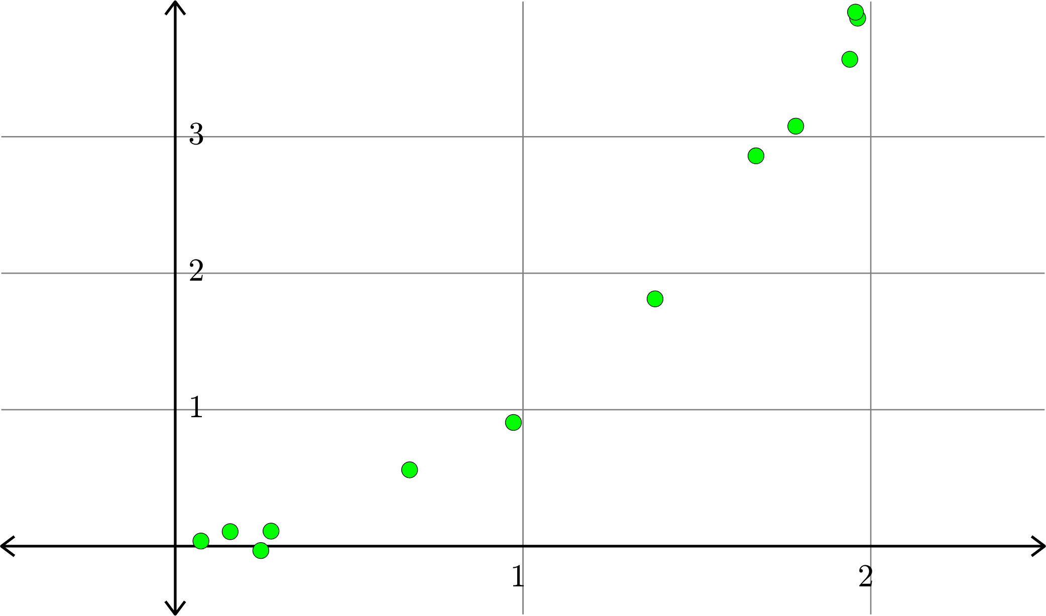
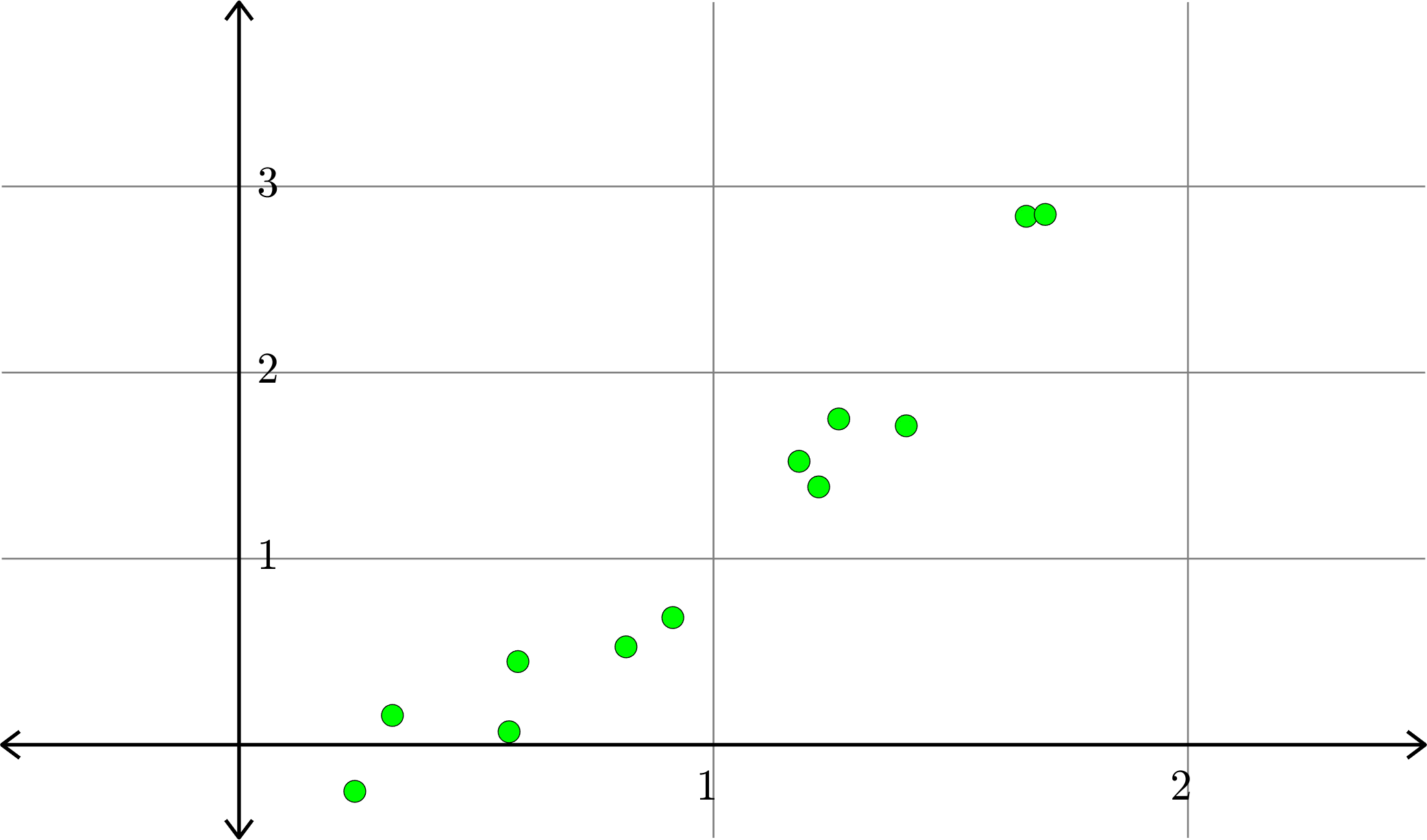
Example. Consider the collection of points in \(\R^{2}\):
\[(x_{1},y_{1}),(x_{2},y_{2}),\ldots,(x_{n},y_{n})\]
We want to find the polynomial \(p(x)\) of degree \(k\) or less such that \(\displaystyle{\sum_{i=1}^{n}|p(x_{i})-y_{i}|^{2}}\) is as small as possible.
\(k=1\)
\(k=1\)
\(k=1\)
\(k=2\)
\(k=2\)
\(k=2\)
Example. Consider the collection of points in \(\R^{2}\):
\[(x_{1},y_{1}),(x_{2},y_{2}),\ldots,(x_{n},y_{n})\]
We want to find the polynomial \(p(x)\) of degree \(k\) or less such that \(\displaystyle{\sum_{i=1}^{n}|p(x_{i})-y_{i}|^{2}}\) is as small as possible.
Set \[A= \begin{bmatrix}1 & x_{1} & x_{1}^{2} & \cdots & x_{1}^{k}\\[1ex] 1 & x_{2} & x_{2}^{2} & \cdots & x_{2}^{k}\\[1ex] 1 & x_{3} & x_{3}^{2} & \cdots & x_{3}^{k}\\ \vdots & \vdots & \vdots & & \vdots \\ 1 & x_{n} & x_{n}^{2} & \cdots & x_{n}^{k}\\\end{bmatrix} \quad\text{and}\quad b= \begin{bmatrix}y_{1}\\ y_{2}\\ y_{3}\\ \vdots\\ y_{n}\end{bmatrix}\]
If \(\hat{x} = \begin{bmatrix} a_{0}\\ a_{1}\\ \vdots\\ a_{k}\end{bmatrix}\) is the least squares solution to \(Ax=b\), then we see that
\[\|A\hat{x} - b\|^{2}\] is as small as possible among all possible \(\hat{x}\).
However
\[A\hat{x}-b = \begin{bmatrix} a_{0}+a_{1}x_{1}+a_{2}x_{1}^{2}+\cdots + a_{k}x_{1}^{k} - y_{1}\\ a_{0}+a_{1}x_{2}+a_{2}x_{2}^{2}+\cdots + a_{k}x_{2}^{k} - y_{2}\\ a_{0}+a_{1}x_{3}+a_{2}x_{3}^{2}+\cdots + a_{k}x_{3}^{k} - y_{3}\\ \vdots\\ a_{0}+a_{1}x_{n}+a_{2}x_{n}^{2}+\cdots + a_{k}x_{n}^{k} - y_{n}\end{bmatrix} = \begin{bmatrix} p(x_{1})-y_{1}\\ p(x_{2})-y_{2}\\ p(x_{3})-y_{3}\\ \vdots\\ p(x_{n})-y_{n}\end{bmatrix}\]
where \[p(x) = a_{0}+a_{1}x+a_{2}x^2+a_{3}x^3+\cdots+a_{k}x^{k}.\]
Therefore,
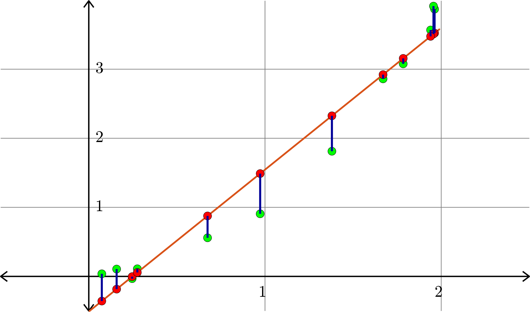
\[\|A\hat{x} - b\|^{2} = \sum_{i=1}^{n}|p(x_{i})-y_{i}|^{2}\]
If \(q(x)\) is any polynomial of degree \(\leq k\), say
\[q(x) = c_{0}+c_{1}x+c_{2}x^2+c_{3}x^3+\cdots+c_{k}x^k.\]
Then we set \[z = \begin{bmatrix} c_{0}\\ c_{1}\\ \vdots\\ c_{k}\end{bmatrix}\]
and we see that
\[\|Az-b\|^{2}\geq \|A\hat{x} - b\|^{2},\]
that is,
\[\sum_{i=1}^{n}|q(x_{i})-y_{i}|^{2}\geq \sum_{I=1}^{n}|p(x_{i})-y_{i}|^{2}\]
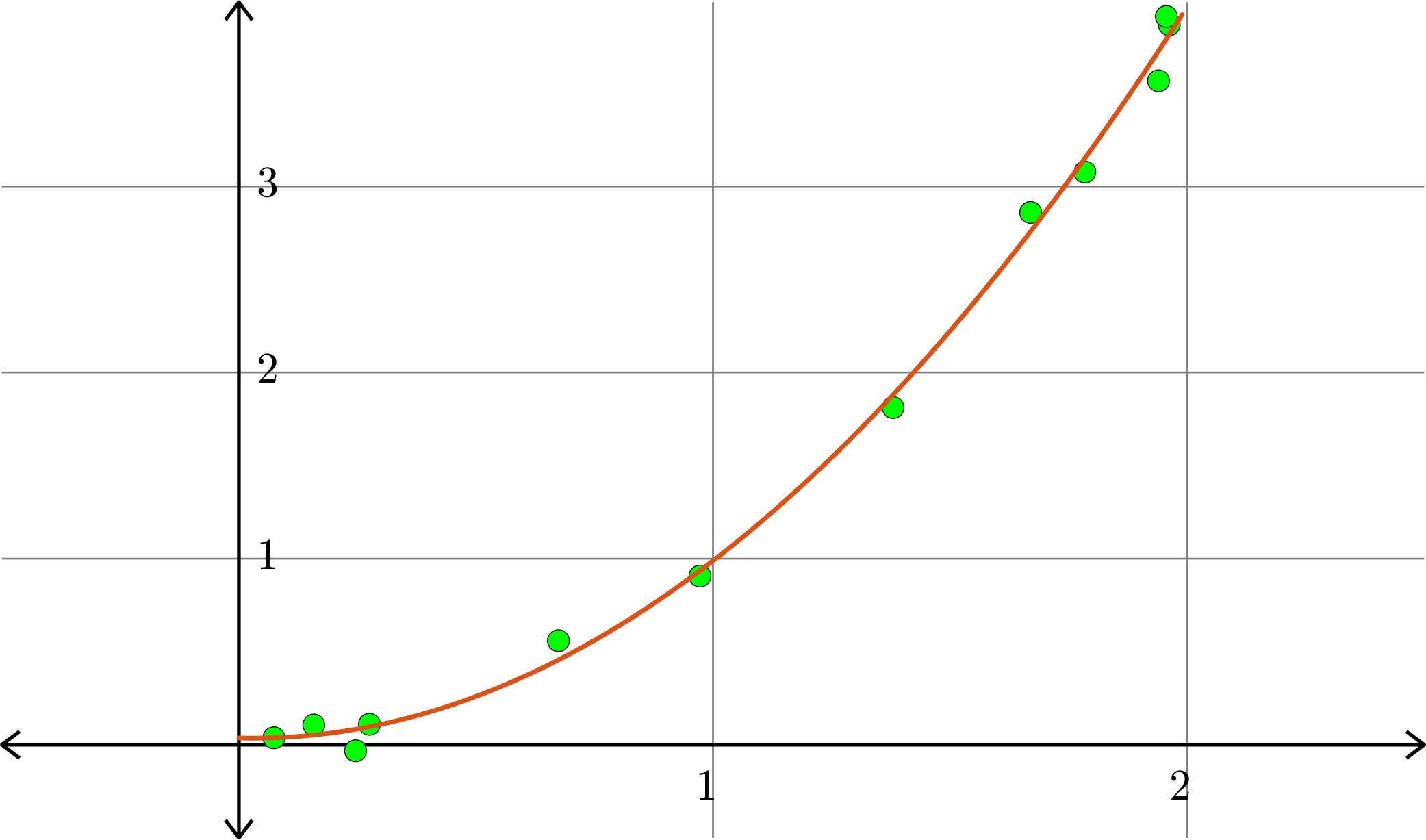
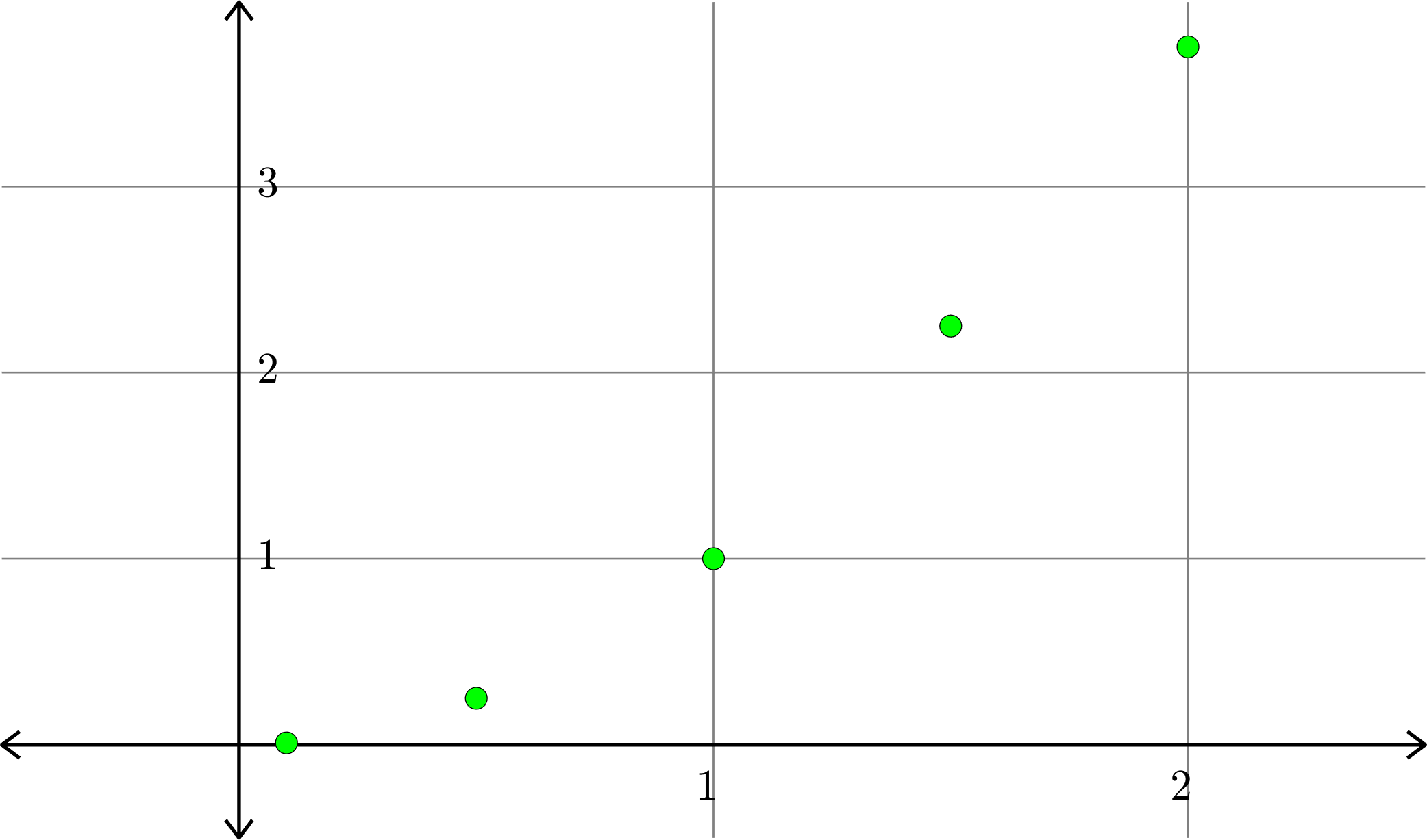
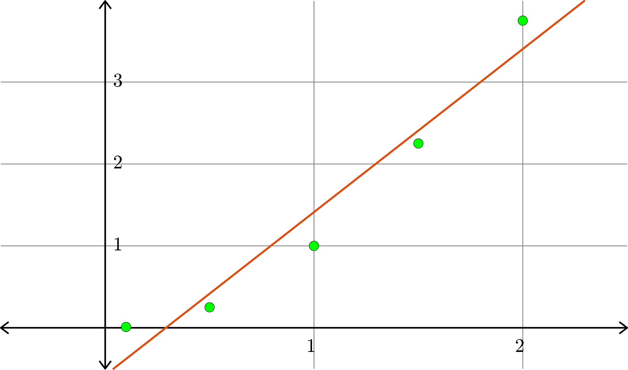
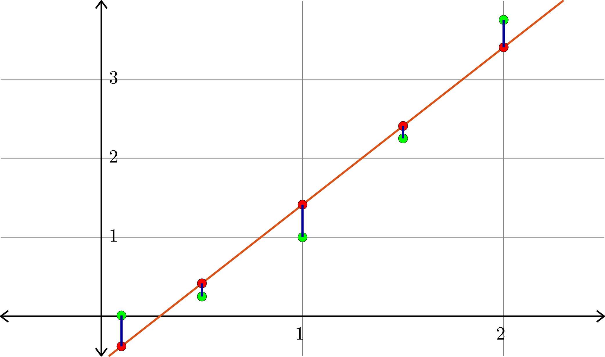
Example. Consider the collection of points in \(\R^{2}\):
\[(1,1), (0.5,0.25), (1.5,2.25),(0.1,0.01),(2,3.75)\]
\[A = \begin{bmatrix} 1 & 1\\ 1 & 0.5\\ 1 & 1.5\\ 1 & 0.1\\ 1 & 2\end{bmatrix}\quad\text{and}\quad b = \begin{bmatrix} 1\\ 0.25\\ 2.25\\ 0.01\\ 3.75\end{bmatrix}\]
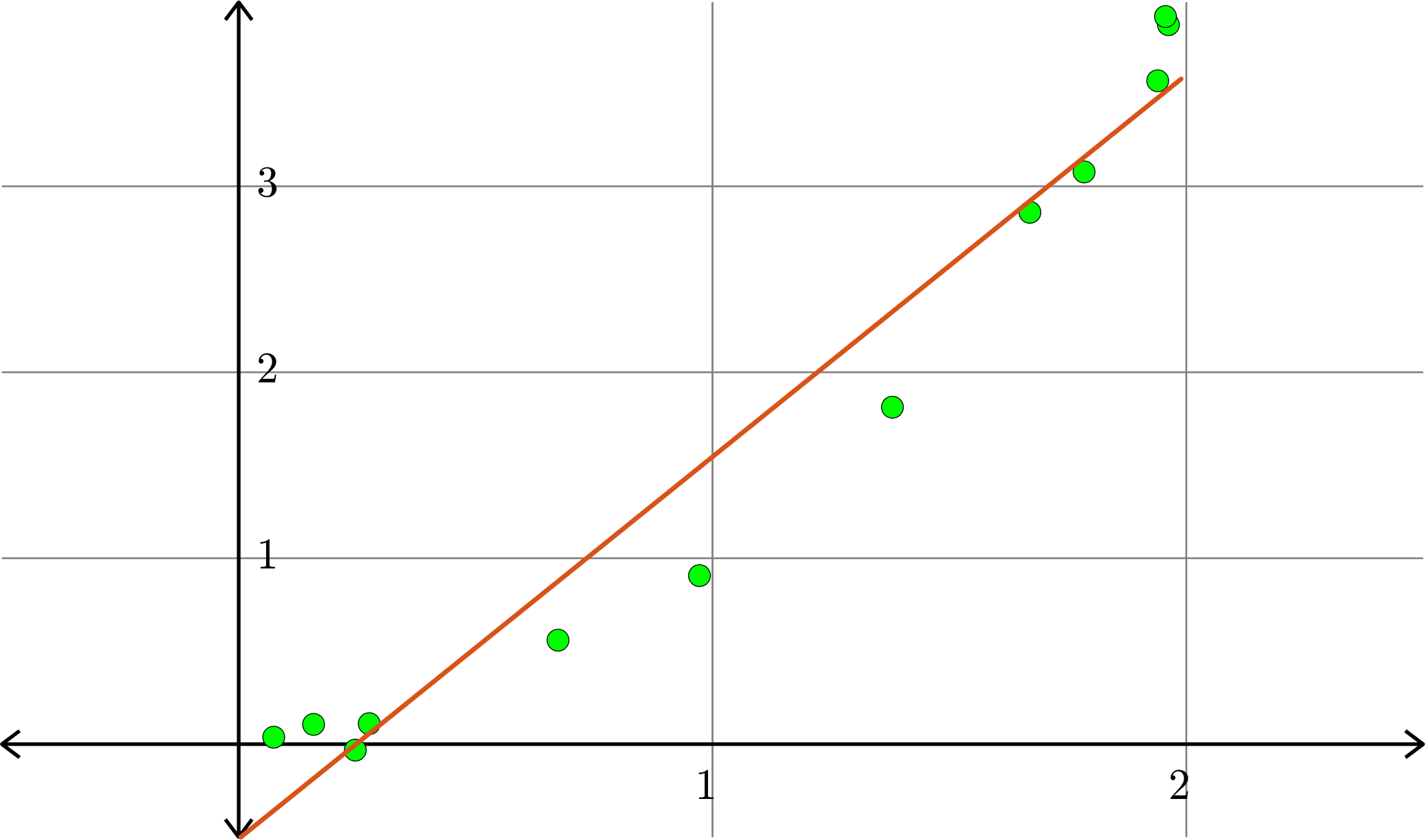
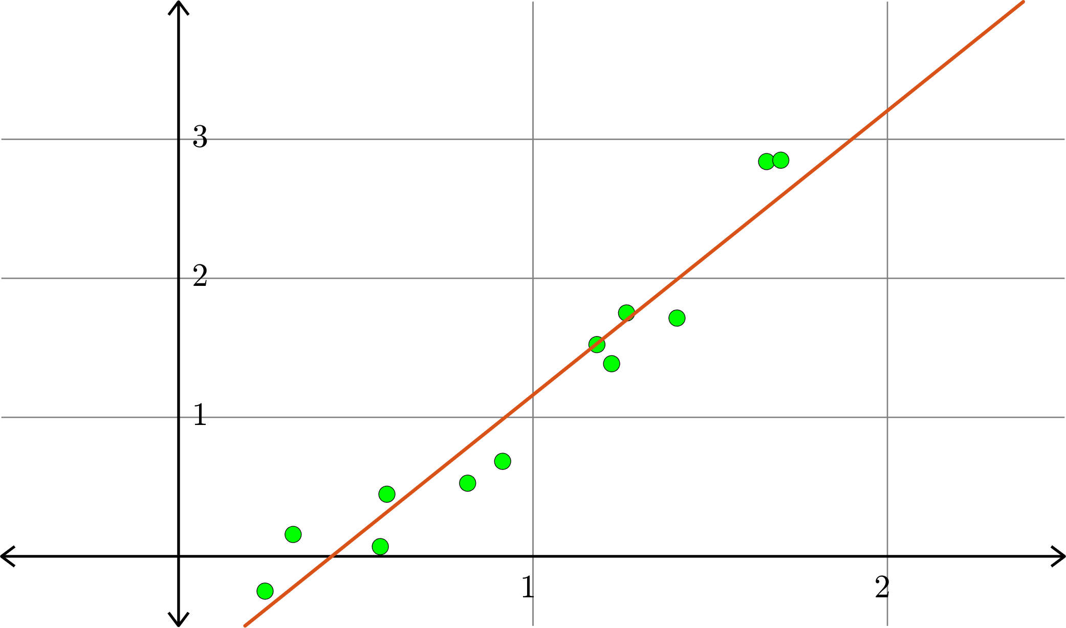
\[\hat{x} = \begin{bmatrix}-0.5791\\ 1.9912\end{bmatrix}\]
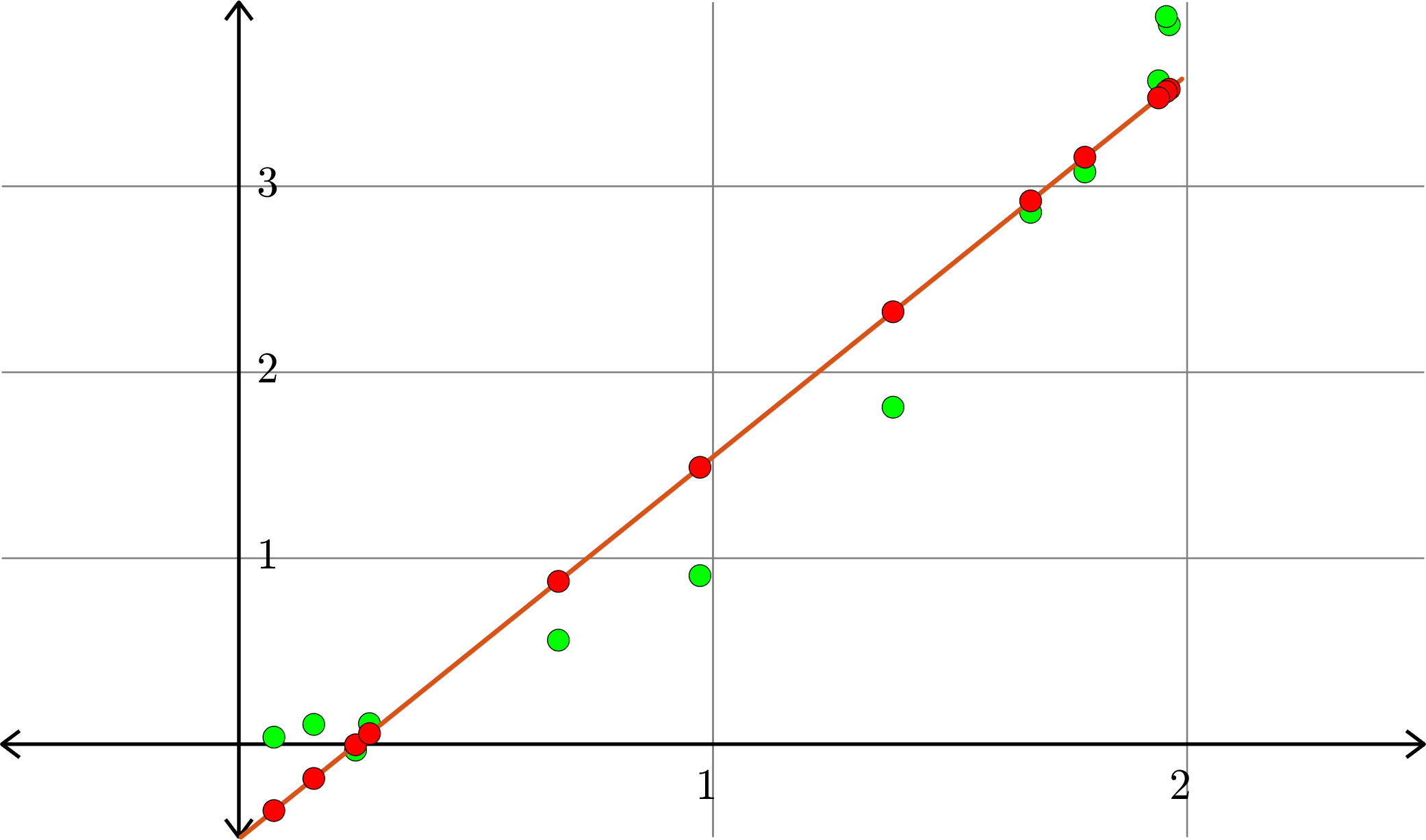
Hence \(p(x) = -0.5791+1.9912x\) is the closest linear (degree 1) polynomial to the points, in the sense stated before.
Degree \(1\):
Example. Consider the collection of points in \(\R^{2}\):
\[(1,1), (0.5,0.25), (1.5,2.25),(0.1,0.01),(2,3.75)\]
Degree \(1\):
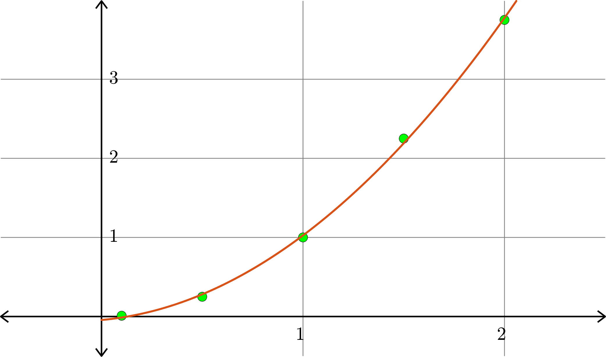
Example. Consider the collection of points in \(\R^{2}\):
\[(1,1), (0.5,0.25), (1.5,2.25),(0.1,0.01),(2,3.75)\]
\[A = \begin{bmatrix} 1 & 1 & 1\\ 1 & 0.5 & 0.25\\ 1 & 1.5 & 2.25\\ 1 & 0.1 & 0.01\\ 1 & 2 & 4\end{bmatrix}\quad\text{and}\quad b = \begin{bmatrix} 1\\ 0.25\\ 2.25\\ 0.01\\ 3.75\end{bmatrix}\]
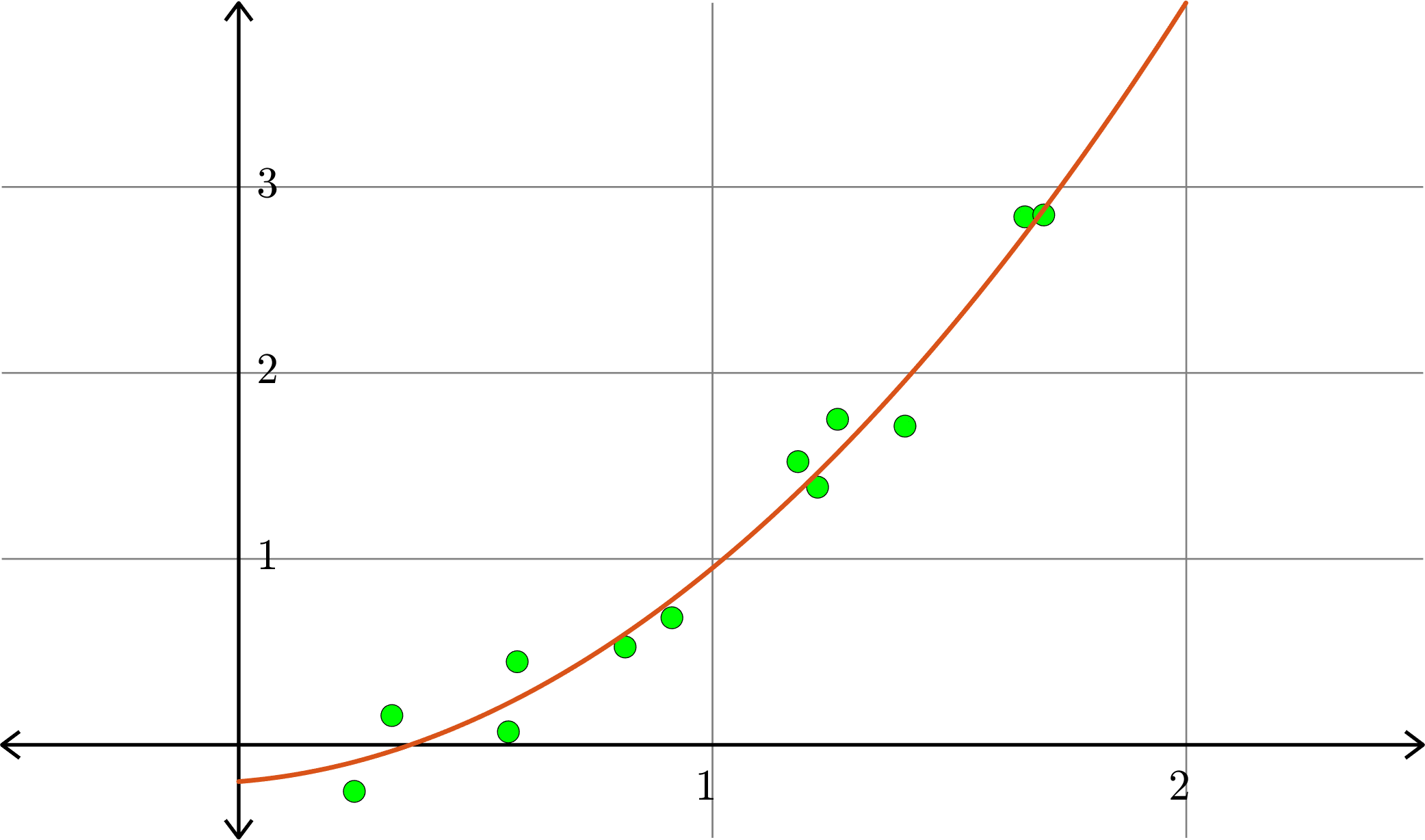
\[\hat{x} = \begin{bmatrix} -0.0436 \\ 0.2292\\ 0.8401\end{bmatrix}\]
Hence \(p(x) = -0.0436+0.2292x+0.8401x^2\) is the closest quadratic (degree 2) polynomial to the points, in the sense stated before.
Degree \(2\):
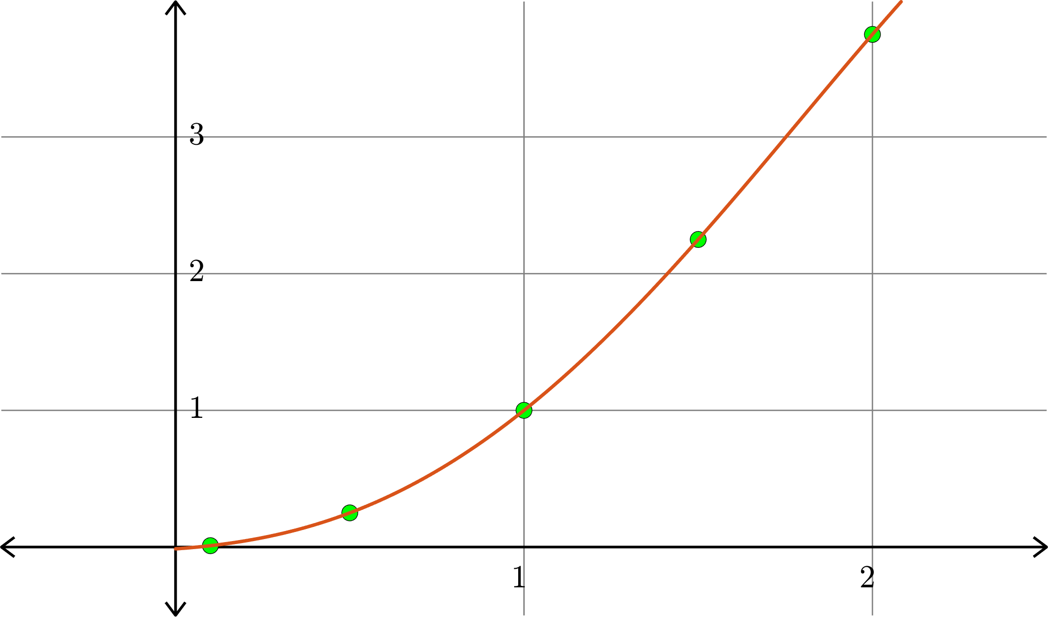
Example. Consider the collection of points in \(\R^{2}\):
\[(1,1), (0.5,0.25), (1.5,2.25),(0.1,0.01),(2,3.75)\]
Degree \(2\):
\(p(x) = -0.0436+0.2292x+0.8401x^2\)
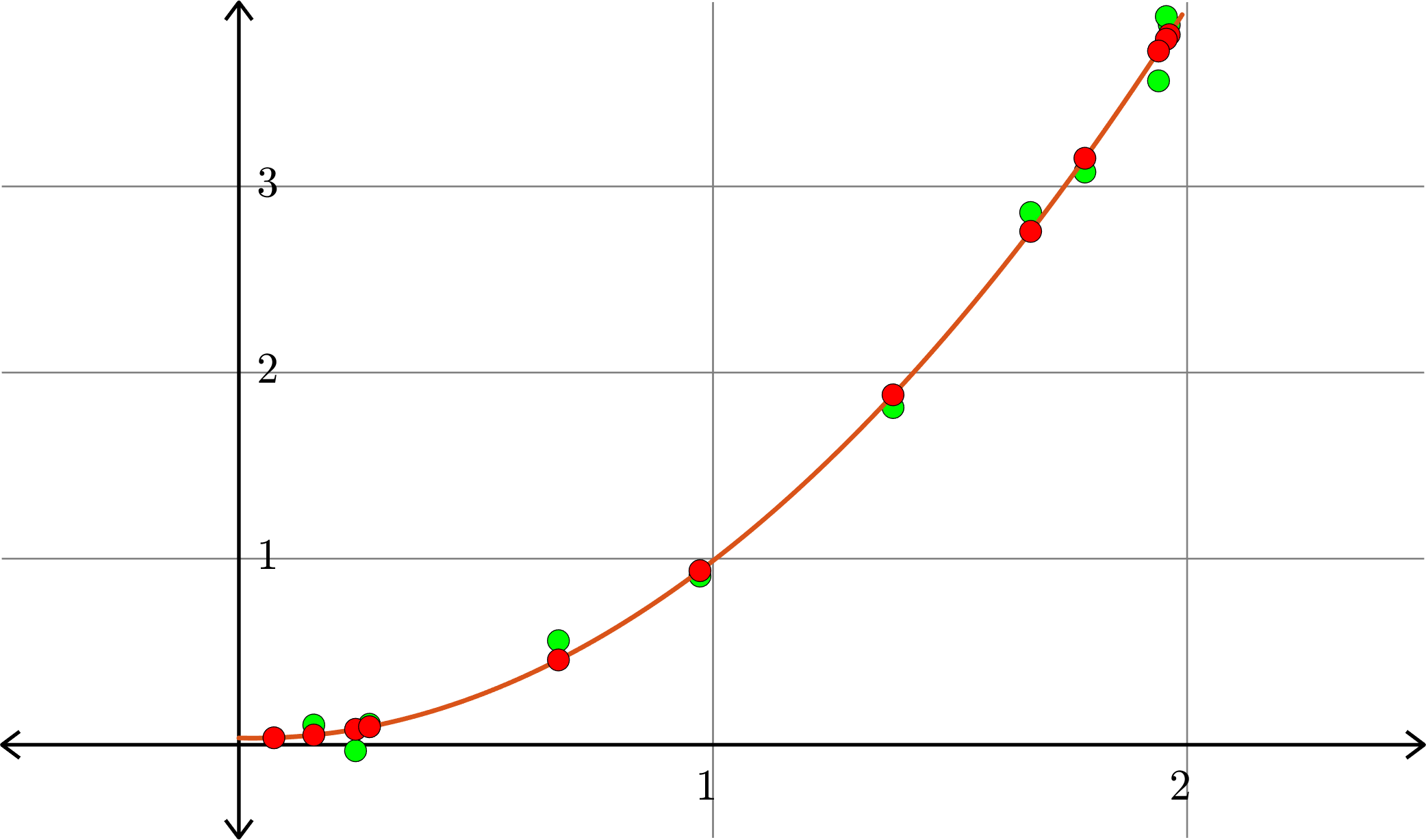
Example. Consider the collection of points in \(\R^{2}\):
\[(1,1), (0.5,0.25), (1.5,2.25),(0.1,0.01),(2,3.75)\]
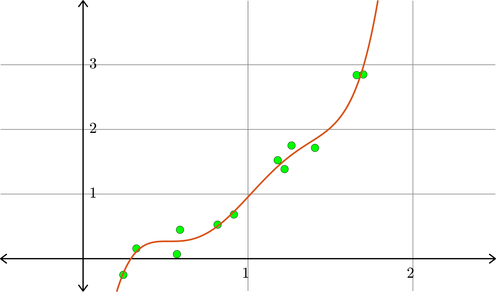
Degree \(3\):

\(p(x) = 0.0248-0.2431x+1.4215x^2-0.1839x^3\)
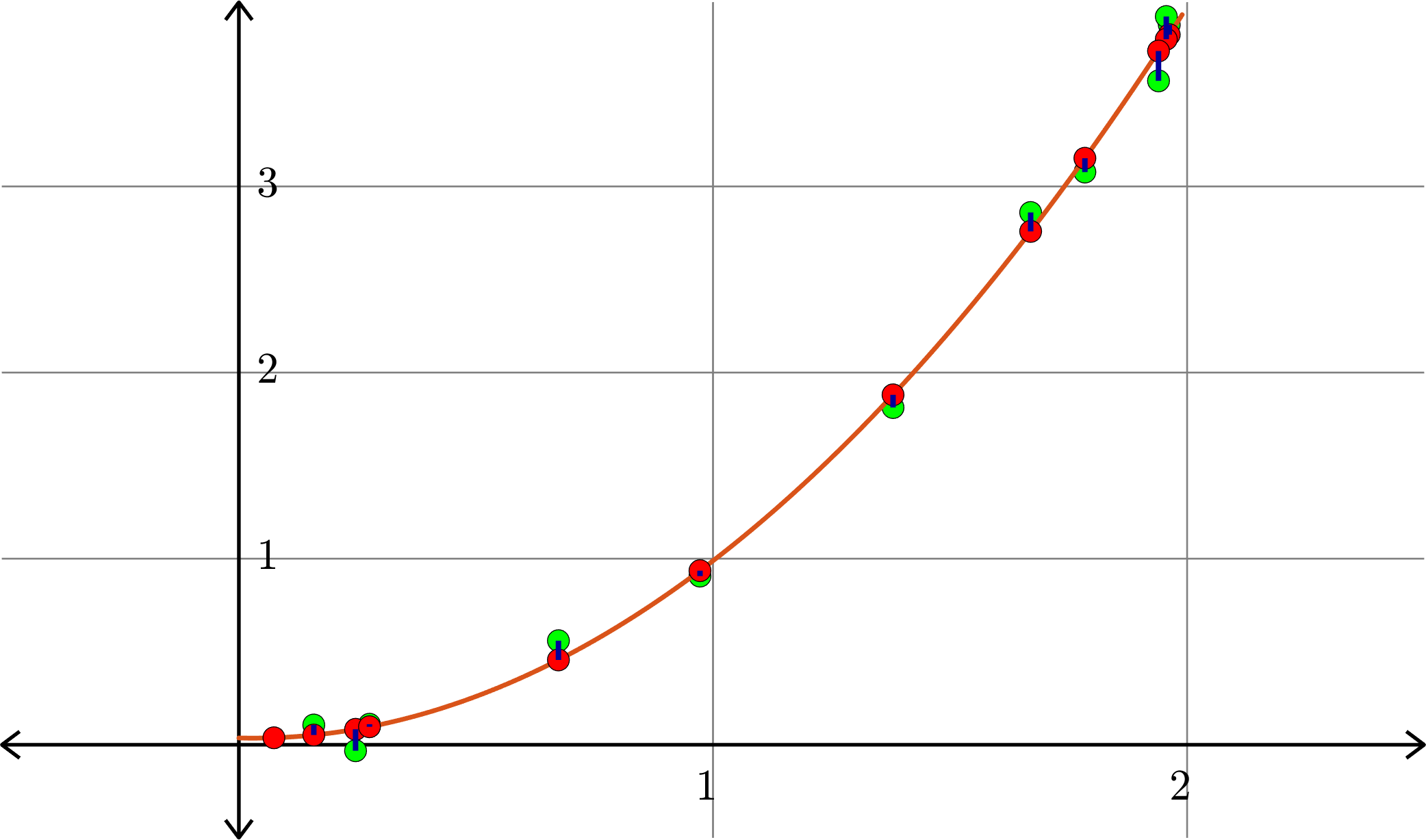
Example. Consider the collection of points in \(\R^{2}\):
\[(1,1), (0.5,0.25), (1.5,2.25),(0.1,0.01),(2,3.75)\]
Degree \(4\):
Example. Consider the collection of points in \(\R^{2}\):
\[(1,1), (0.5,0.25), (1.5,2.25),(0.1,0.01),(2,3.75)\]
Degree \(5\):

Example. Consider the collection of points in \(\R^{2}\):
Example. Consider the collection of points in \(\R^{2}\):
Linear polynomial (degree 1)
Example. Consider the collection of points in \(\R^{2}\):
Quadratic polynomial (degree 2)
Example. Consider the collection of points in \(\R^{2}\):
Degree \(5\) polynomial
Example. Consider the collection of points in \(\R^{2}\):
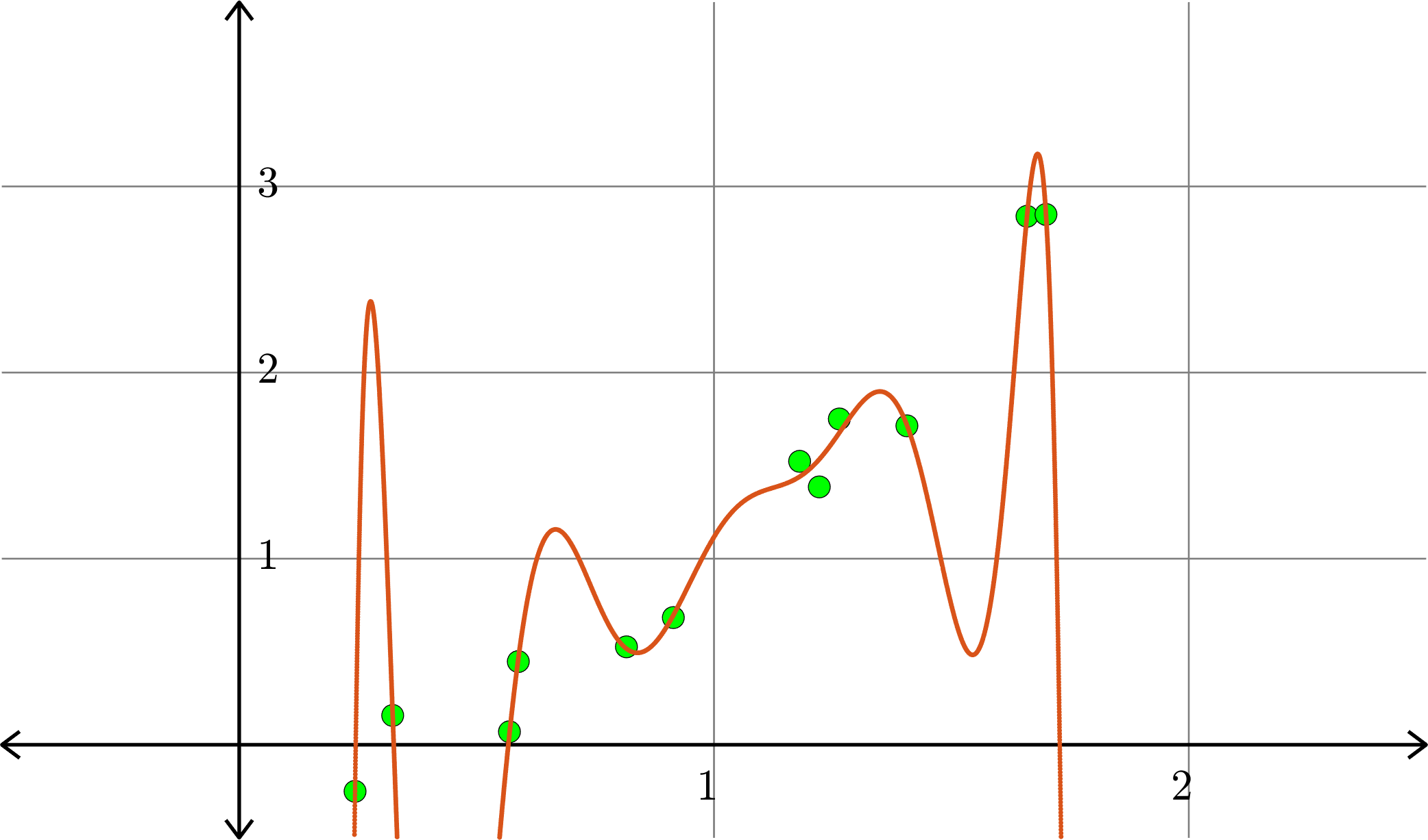
Degree \(10\) polynomial
Example. Consider the collection of points in \(\R^{2}\):
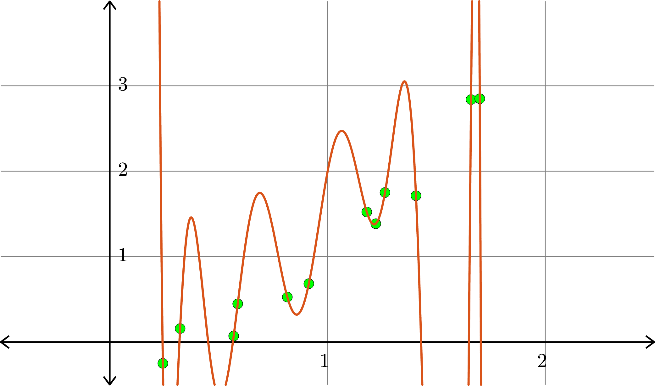
Degree \(11\) polynomial
Linear Algebra Day 32
By John Jasper


