Real Analysis

Part 1:

Sets

(See Chapter 1 in Book of Proof)

The central objects in mathematics are sets. A set is a collection of things. The things in a set are called elements.

Sets

Often, we denote a set by simply writing all the elements between \(\{\}\) ("curly braces") separated by commas. For example,

\[\{1,2,4,5\}\]

is the set with four elements, these elements being \(1,2,4,\) and \(5\).

We often give sets names, these will frequently be a single capital roman letter, for example, \[B = \{1,2,4,5\}.\]

To express the statement "\(x\) is an element of \(A\)" we write \(x\in A\). Thus, given the set \(B\) defined above, we see that \(1\in B\) is a true statement, and \(3\in B\) is a false statement.

We will also write \(x\notin A\) to for the statement "\(x\) is not an element of \(A\)."

Equality of sets

Two sets \(A\) and \(B\) are equal (they are the same set) if they contain exactly the same elements, that is, the following two statements hold:

If \(x\in A\), then \(x\in B\).

If \(x\in B\), then \(x\in A\).

In this case we write \(A=B\).

Important example:

Important example: Consider the sets \(A=\{1,2,2,3\}\) and \(B=\{1,2,3\}\). We can easily see that every element of \(A\) is an element of \(B\), and every element of \(B\) is an element of \(A\). Thus

\[\{1,2,2,3\}=\{1,2,3\}.\]

An element is either in a set or it is not. Sets cannot contain multiple copies of an element.

Subsets

Given two sets \(A\) and \(B\), if every element of \(A\) is also an element of \(B\), then we say that \(A\) is a subset of \(B\), and write \(A\subset B\) or \(A\subseteq B\) (these both mean the exact same thing). For example,

\[\{1,2\}\subset\{1,2,4,5\}\]

but \(\{1,2,3\}\) is not a subset of \(\{1,2,4,5\}\) since \(3\in\{1,2,3\}\) and \(3\notin\{1,2,4,5\}\)

Note that the statement "\(A=B\)" can be rewritten as "\(A\subset B\) and \(B\subset A.\)" This will be very useful later.

Ellipsis notation

The set of integers is denoted \(\mathbb{Z}\). The set of positive integers, also called the natural numbers or the naturals, is denoted \(\mathbb{N}\) or \(\mathbb{Z}^{+}\). 

We will sometimes write sets like \(\mathbb{N}\) and \(\mathbb{Z}\) with ellipsis notation, as follows,

\[\N=\{1,2,3,\ldots\}\qquad \Z = \{\ldots,-2,-1,0,1,2,3,\ldots\}\]

In this notation, we list the first several elements of a set, until there is an apparent pattern, then write an ellipsis (...). After the ellipsis we write the final element in the pattern. If no element is written after the ellipsis, then the list of elements goes on without end.

Examples.

• \(\{2,4,6,8,\ldots\}\) is the set of even positive integers.
• \(\{3,7,11,15,\ldots,43\}=\{3,5,7,11,15,19,23,27,31,35,39,43\}\)

Problems with ellipsis notation

Consider the set

\[C:=\{2,4,8,\ldots\}.\]

Questions:

Is \(16\in C\)?    Is \(14\in C\)?

What is the pattern? Is the \(n\)th term in the sequence \(2^{n}\) or \(n^2-n+2\) or something else?

It's not clear!

Suppose \(N\in\mathbb{N}\) and define the set

\[D:=\{2,4,6,\ldots,2N\}.\] If \(N=5\), then

\[D = \{2,4,6,\ldots,10\}=\{2,4,6,8,10\}\]

but if \(N=2\), then

\[D = \{2,4,6,\ldots,4\}(?)\]

We will interpret this set as \(\{2,4\}\). 

Set builder notation

Let \(A\) be a set, and \(S(x)\) denote a statement whose truth value depends on \(x\in A\). The set of \(x\in A\) such that \(S(x)\) is true is denoted

\[\{x\in A : S(x)\}\quad\text{or}\quad \{x\in A\mid  S(x)\}\quad\text{or}\quad \{x : x\in A\text{ and }S(x)\}.\]

Both the colon and the vertical line are read as "such that" or "with the property that."

Example. Consider the set of even positive integers:

\[\{x\in\mathbb{N} : x\text{ is even}\}.\]

This would be read:

"The set of \(x\) in the natural numbers such that \(x\) is even."

Using the notation from the above definition we have \(A=\N\) and \(S(x)\) is the statement "\(x\) is even"

Set builder notation

More generally, let \(A\) be a set. For each \(x\in A\) let \(f(x)\) be an expression that depends on \(x\) and \(S(x)\) denote a statement whose truth value depends on \(x\in A\). The set of all elements of the form \(f(x)\) with the property that \(x\in A\) and \(S(x)\) is true is denoted

\[\{f(x) : x\in A\text{ and }S(x)\}.\]

Example. Consider the set of even positive integers:

\[\{2x: x\in \N\}.\]

In the notation of the above definition we have  \(A=\N\), \(f(x) = 2x\), and \(S(x)\) is true for all \(x\in\N\).

Using set builder notation we can disambiguate the sets from two slides prior:

\[\{2^{n} : n\in\mathbb{N}\}\quad\text{and}\quad\{n^2-n+2 : n\in\mathbb{N}\}.\]

Examples. 

• \(\{2n-1 : n\in\N\text{ and }n\leq 5\} = \{1,3,5,7,9\}\)
• \(\{25-4n : n\in\N\text{ and }n\leq 10\text{ and } n>5\} = \{1,-3,-7,-11,-15\}\)

Consider the set 

\[\{x\in\mathbb{R} : x^{2}+1 = 0\}.\]

There does not exist a real number \(x\) such that \(x^{2}+1=0\), and hence this set does not contain any elements!

The set containing no elements is called the empty set. The empty set is denoted \(\varnothing\) or \(\{\}\).

Part 2:

Proofs and Logic

(See Chapters 2,4,5 & 6 in Book of Proof)

Proposition 1. \(\{n\in\mathbb{Z} : n+1\text{ is odd}\} = \{2n : n\in\mathbb{Z}\}.\)

Proving sets are equal.

Proof. First we will show that \(\{n\in\mathbb{Z} : n+1\text{ is odd}\} \subset \{2n : n\in\mathbb{Z}\}.\) Let \(m\in\{n\in\mathbb{Z} : n+1\text{ is odd}\}\) be arbitrary. This implies that \(m+1\) is odd, that is, there exists \(k\in\Z\) such that \(m+1=2k+1.\) Subtracting \(1\) from both sides we deduce \(m=2k\), and hence \(m\in \{2n : n\in\Z\}.\)

Next, we will show \(\{2n:n\in\mathbb{Z}\}\subset\{n\in\mathbb{Z} : n+1\text{ is odd}\}\).

Let \(p\in\{2n:n\in\mathbb{Z}\}\) be arbitrary. Then, there exists \(q\in\mathbb{Z}\) such that \(p=2q\), and hence \[p+1 = 2q+1.\] Since \(q\in\mathbb{Z}\), we conclude that \(p+1\) is odd, and hence

\(p\in\{n\in\mathbb{Z} : n+1\text{ is odd}\}.\) \(\Box\)

Definition. An integer \(n\) is even if there exists an integer \(k\) such that \(n=2k\). An integer \(n\) is odd if there exists an integer \(p\) such that \(n=2p+1\).

Proposition 2. If \(n\in\Z\) is odd, then \(n^{2}\) is odd.

Proving implications (Direct proof)

\(A : n\) is odd

\(B : n^{2}\) is odd

We wish to prove the implication \(A\Rightarrow B\). We will use a direct proof, that is, we will assume \(A\), argue directly to \(B\).

Proof. Suppose \(n\in\Z\) is odd. By definition, this means that there exists \(k\in\Z\) such that \(n=2k+1\). This implies

\[n^{2} = (2k+1)^{2} = 4k^{2}+4k+1 = 2(2k^{2}+2k)+1.\]

Since \(2k^{2}+2k\) is an integer, we conclude that \(n^{2}\) is odd. \(\Box\)

Proposition 3. Suppose \(n\in\Z\). If \(n^{2}\) is even, then \(n\) is even.

Proving implications (Contrapositive proof)

Proposition 4. Suppose \(a,b,c\in\Z\). If \(a^{2}+b^{2}=c^{2}\), then either \(a\) is even or \(b\) is even.

Proving implications (Proof by contradiction)

Proposition 4. Suppose \(a,b,c\in\Z\). If \(a^{2}+b^{2}=c^{2}\), then either \(a\) is even or \(b\) is even.

Proposition 3. Suppose \(n\in\Z\). If \(n^{2}\) is even, then \(n\) is even.

Contrapositive vs. Contradiction

Proof. Assume toward a contradiction that \(n\) is not even and \(n^{2}\) is even. This implies that \(n\) is odd, that is \(n=2k+1\) for some \(k\in\Z\). Squaring, we obtain

\[n^{2} = 4k^{2}+4k+1=2(2k^{2}+2k)+1.\]

Since \(2k^{2}+2k\) is an integer, this shows that \(n^{2}\) is odd. This contradicts the fact that \(n^{2}\) is even.\(\Box\)

Proof by contradiction: \(A\wedge(\sim\!B)\Rightarrow C\wedge(\sim\!C)\)

Contrapositive: \((\sim\!B)\Rightarrow(\sim\!A)\)

Fake proof by contradiciton: \(A\wedge(\sim\!B)\Rightarrow A\wedge(\sim\!A)\)

Moral: If your proof by contradiction concludes with \(\sim\!A\), then you should use proof by contrapositive instead!

Universal quantifier

\(A : n^{2}\) is even

\(B : n\) is even

Note that \(A\) and \(B\) below are not statements. They're truth value depends on \(n\).

These are more precisely called open sentences (or predicates or propositional functions). They should really have variables

\(A(n) : n^{2}\) is even

\(B(n) : n\) is even

Proposition 3. Suppose \(n\in\Z\). If \(n^{2}\) is even, then \(n\) is even.

Recall the proposition:

Now, Proposition 3 can be more precisely written as \[\forall\,n\in\Z,\ A(n)\Rightarrow B(n).\]

Where the symbol \(\forall\) stands for "for all" or "for every," and is called the universal quantifier.

Note that \(A(n) : n^{2}\) is even, is false unless \(n\in\Z\).

Recall that for false statements \(A\), the statement \(A\Rightarrow B\) is true for any statement \(B\). (In this case \(A\Rightarrow B\) is called a vacuously true statement.)

Thus, in the statement \(\forall\,n\in\Z,\ A(n)\Rightarrow B(n)\) the universal quantifier isn't really necessary. It would be very common to see Proposition 3 written as

Proposition 3. If \(n^{2}\) is even, then \(n\) is even.

The universal quantifier "For all \(n\in\Z\)" is there, it's just not written.

Moral: In math we often omit the universal quantifier before an implication.

Existential quantifier

To say that an open sentence \(A(x)\) is true for all \(x\) in a set \(X\) we use the universal quantifier:

\[\forall\,x\in X,\ A(x).\]

In math, we would write this using words:

"For all \(x\in X\), \(A(x)\) is true."

To say that an open sentence \(A(x)\) is true for at least one \(x\) in a set \(X\) we use the existential quantifier \[\exists\, x\in X,\ A(x).\] In words:

"There exists \(x\in X\) such that \(A(x)\) is true."

Universally quantified statements may be more common, but here is an example of a statement that is not:

"The polynomial \(x^{5}+5x^3+10\) has a real root."

Do you see that this statement is of the form \(\exists\, x\in X,\ A(x)\). What are the set \(X\) and the open sentence \(A(x)\)?

Order of quantifiers

Consider the following two statements:

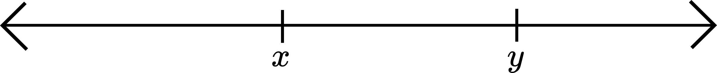
\(A:\ \) For every even \(n\in\N\) there exists an odd \(m\in\N\) such that \(m>n\).

\(B:\ \) There exists odd \(m\in\N\) such that for all even \(n\in\N\), it is true that \(m>n\).

Because it sounds better in English, we will often write \(B\) as

\(B:\ \) There exists odd \(m\in\N\) such that \(m>n\) for all even \(n\in\N\).

Let \(E\) denote the set of even natrual numbers, and let \(D\) denote the set of odd natural numbers. Using symbols, we can write \(A\) and \(B\) as follows: \[A: \forall\, n\in E,\ \exists\,m\in D,\ m>n\]

\[B: \exists\,m\in D,\ \forall\, n\in E,\ m>n\]

Moral: \(A\) is true, and \(B\) is false. The order of the quantifiers matters. You must think hard to figure out the meaning of a statement, there is no shortcut!

Proving universally quantified statements

Every universally quantified statement can be converted to an implication:

\[\forall\, x\in X,\ A(x)\]

is the same as

\[(x\in X)\Rightarrow A(x)\]

Thus, to prove this statement we take an "arbitrary" element \(x\in X\), then reason that \(A(x)\) is true for that \(x\). The proof looks like

Proof. Let \(x\in X\) be arbitrary.

\[\vdots\]

\[\vdots\]

Therefore, \(A(x)\). \(\Box\)

For example, let's say we want to prove the following statement:

Proposition. For every even number \(n\in\N\), the number \(n^2+1\) is odd.

For example, let's say we want to prove the following statement:

Proposition. For every even number \(n\in\N\), the number \(n^2+1\) is odd.

Proof. Let \(n\in\N\) be an arbitrary even number. This implies that \(n=2k\) for some integer \(k\), and thus

\[n^2+1 = (2k)^{2}+1 = 4k^{2}+1 = 2(2k^{2})+1.\]

Since \(2k^2\) is an integer, we conclude that \(n^2+1\) is odd. \(\Box\)

Proving quantified statements

Theorem 1.18. For every positive real number \(x\) there exists a natural number \(n\) such that \(n>x.\)

Proposition. For every \(\varepsilon>0\) there exists \(m\in\N\) such that \(\dfrac{1}{m}<\varepsilon\).

The following is an important property of the natural numbers and the real numbers. We will prove it later, but for now we will assume it is true.

Proving quantified statements

Proposition. For every \(\varepsilon>0\) there exists \(m\in\N\) such that \(\dfrac{1}{m}<\varepsilon\).

What would it look like if we tried to prove this statement by contradiction?

Statement: \(\forall\,\varepsilon>0,\ \exists\,m\in\N,\ \dfrac{1}{m}<\varepsilon.\)

Negation: \(\exists\,\varepsilon>0,\ \forall\,m\in\N,\ \dfrac{1}{m}\geq\varepsilon.\)

In words, the negation might read:

There exists \(\varepsilon>0\) such that \(\varepsilon\leq \dfrac{1}{m}\) for all \(m\in\mathbb{N}\).

Part 3:

Real numbers

(See sections 1.1-1.19 in Apostol)

The Real Numbers

The real numbers is the set denoted \(\mathbb{R}\) with two binary operations, addition and multiplication, and a relation \(<\), that satisfy the following ten axioms.

Axiom 1. \(x+y=y+x\), \(xy=yx\)

Axiom 2. \(x+(y+z)=(x+y)+z\), \(x(yz)=(xy)z\)

Axiom 3. \(x(y+z) = xy+xz\)

Axiom 4. For all \(x,y\in\mathbb{R}\), there exists a unique number \(z\in\mathbb{R}\) such that \(x+z=y\). This number \(z\) is denoted \(y-x\), and \(x-x\) is denoted \(0\). We also write \(-x\) for \(0-x\).

(commutative laws)

(associative laws)

(distributive law)

The order axioms

Axiom 6.  For \(x,y\in\R\) exactly one of the following is true:

\[x<y,\ y<x,\text{ or }x=y.\]

Axiom 7. If \(x<y\), then \(x+z<y+z\) for all \(z\in\mathbb{R}\).

Axiom 8. If \(x>0\) and \(y>0\), then \(xy>0\).

Axiom 9. If \(x>y\) and \(y>z\), then \(x>z\).

Note that \(x>y\) means \(y<x\). (That had to be stated?! Yep!) If \(x>0\) then we say that \(x\) is positive. We write \(x\leq y\) for the statement

\[x<y\text{  or  }x=y,\]

and similarly for \(x\geq y\). If \(x\geq 0\) then we say that \(x\) is nonnegative. If \(x<0\) then we say that \(x\) is negative. If \(x\leq 0\) then we say that \(x\) is nonpositive.

Before we state Axiom 10, the completeness axiom, let's look at some consequences of the first nine axioms.

Proposition 2. If \(x,y,z\in\mathbb{R}\), then \(x(y-z)=xy-xz\).

Proposition 5. \(1>0\).

Proposition 6.  If \(a<b\) and \(c>0\), then \(ac<bc\).

The rational numbers

The integers are the numbers in set

\[\mathbb{Z}:=\N\cup\{0\}\cup\{-n : n\in\mathbb{N}\}.\]

The rational numbers are the numbers in the set

\[\mathbb{Q} = \left\{\frac{m}{n} : m,n\in\Z\text{ and }n\neq 0\right\}.\]

If \(x\in\mathbb{R}\setminus\mathbb{Q}\), that is, \(x\) is a real number which is not a rational number, then \(x\) is called an irrational number.

Theorem. There does not exist \(x\in\mathbb{Q}\) such that \(x^{2} = 2\).

Proof. See Theorem 1.10 in the text. \(\Box\)

Note that it would be incorrect at this point to say that \(\sqrt{2}\notin\mathbb{Q}\) since we do not know that there is a real number \(x\) such that \(x^{2} = 2\).

Upper bounds

Definition 1.12. Let \(S\) be a set of real numbers. If there is a real number \(b\) such that \(x\leq b\) for all \(x\in S\), then \(b\) is called an upper bound for \(S\) and we say that \(S\) is bounded above by \(b\). If \(S\) has no upper bound, then we say that \(S\) is unbounded above.

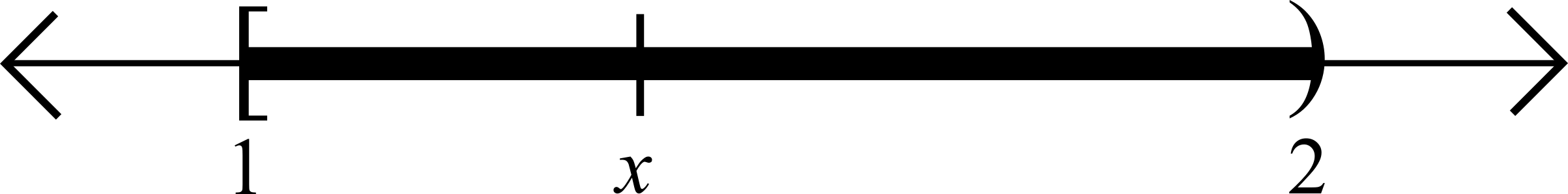
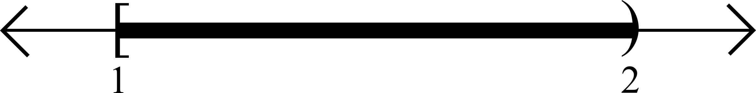
The interval \[[1,2)=\{x : 1\leq x<2\}\] is bounded above by \(2\).

It is also bounded above by \(138\).

It is not bounded above by \(3/2,\) since \(7/4\in[1,2),\) but \(7/4>3/2\).

Note that \(2\) is an upper bound, but any number less than \(2\) is not an upper bound. So \(2\) is the least upper bound for \([1,2)\).

In fact, a number \(x\) is an upper bound for \([1,2)\) if and only if \(x\geq 2\). Thus, the set \([1,2)\) does not contain any upper bounds for itself.

Maximum elements

If set \(S\subset\mathbb{R}\) and there exists \(b\in S\) such that \(b\) is an upper bound for \(S\), then \(b\) is called the maximum element or largest element of \(S\). In this case we write

\[b=\max S.\]

Examples. 

1. The set \([1,2)\) does not have a maximum element.
2. The set \((1,2]\) does have a maximum element, namely, \(\max(1,2]=2.\)
3. The empty set \(\varnothing\) has no maximum elements, but every real number is an upper bound.

Proposition 9. \([1,2)\) does not have a maximum element.

Proposition 9. \([1,2)\) does not have a maximum element.

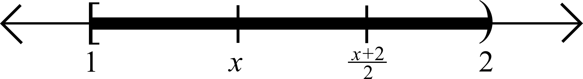
Proof. We will show that if \(x\in[1,2)\), then \(x\) is not an upper bound for \([1,2)\). Let \(x\in [1,2)\) be arbitrary. Define the number \[y=\dfrac{x+2}{2}.\]

Note that

\[x=\frac{x+x}{2}<\frac{x+2}{2}<\frac{2+2}{2}=2\]

and

\[\frac{x+2}{2}\geq \frac{1+2}{2}=\frac{3}{2}.\]

This shows that \(y\in[1,2)\) and \(y>x\). \(\Box\)

Supremum and infimum

Definition 1.13. Let \(S\subset\mathbb{R}\) be bounded above. A real number \(b\) is called a least upper bound for \(S\) if it has the following two properties:

a) \(b\) is an upper bound for \(S\).

b) No number less than \(b\) is an upper bound for \(S\).

A least upper bound for \(S\) is also called a supremum. If \(b\) is a supremum for \(S\), then we write \[b=\sup S.\]

Proposition 10. If \(S\subset\mathbb{R}\) has a supremum, then it is unique. 

Proof. Suppose \(a\) and \(b\) are both least upper bounds for \(S\). If \(a\) and \(b\) are not equal, then either \(a<b\) or \(b<a\). Since both \(a\) and \(b\) are upper bounds for \(S\), both \(a<b\) and \(b<a\) contradict the assumption about \(a\) and \(b\) in Definition 1.13 (b). \(\Box\)

Proposition 11. \(\sup[1,2)=2\).

Proof. It is clear that \(2\) is an upper bound for \([1,2)\). Let \(b<2\) be arbitrary. If \(b<1\), then \(b\) is not an upper bound since \(1\in[1,2)\). For \(b\geq 1\), as in the proof of Proposition 9 we see that \(y=\frac{b+2}{2}\in[1,2)\) and \(y>b\). This shows that \(b\) is not an upper bound for \([1,2)\), that is, there is no upper bound for \([1,2)\) less than \(2\). \(\Box\)

The completeness axiom

Axiom 10. Every nonempty set \(S\subset\mathbb{R}\) which is bounded above has a supremum.

Theorem 1.14 (Approximation property). Let \(S\) be a nonempty set of real numbers with a supremum, say \(b=\sup S\). Then, for every \(a<b\) there exists \(x\in S\) such that \(a<x\leq b\).

Proof. (On the board and in the text).

Theorem 1.15 (Additive property). Given nonempty sets \(A,B\subset\mathbb{R}\), let \(C\) denote the set

\[C:=\{x+y : x\in A,\ y\in B\}.\]

If \(A\) and \(B\) both have supremums, then \(C\) has a supremum, and

\[\sup C = \sup A+\sup B\]

Proof. (On the board and in the text).

Theorem 12. There is a positive real number \(b\) such that \(b^{2}=2\). We will call this number \(\sqrt{2}\).

Proof. (On the board). \(\Box\)

We have already shown that \(\sqrt{2}\) is not rational, thus there exist numbers in \(\R\setminus\mathbb{Q}\). Such numbers are called irrational numbers.

Theorem 1.10. If \(n\) is a positive integer which is not a perfect square, then \(\sqrt{n}\) is irrational.

In the book it is proven that there is no rational number \(a\) such that \(a^{2} = n\). It can be proven by a similar argument to the above theorem that there is a real number \(a\) such that \(a^{2}=n\).

Theorem 1.17. The set \(\mathbb{N}\) of positive integers is unbounded above.

Theorem 1.18. For every positive real number \(x\) there exists a natural number \(n\) such that \(n>x.\)

Theorem 1.19 (The Archimedian property of \(\mathbb{R}\)). If \(x>0\) and \(y\in\mathbb{R}\), then there exists \(n\in\mathbb{N}\) such that \(nx>y\).

Integers and completeness

Assuming Theorem 1.17 we see that Theorem 1.18 is essentially a restatement of Theorem 1.18.

Assuming Theorem 1.18, given \(x>0\) and \(y\in\mathbb{R}\) we apply Theorem 1.18 to \(y/x\) to obtain \(n\in\mathbb{N}\) such that \(n>y/x\), then multiply both sides by \(x\).

Theorem 13. Every nonempty set \(X\subset\mathbb{N}\) has a minimal element.

Proof. Since \(X\) is nonempty and bounded below by \(1\) by HW3 Problem 1 we see that \(X\) has an infimum, say \(m=\inf X\).

By Theorem 1.14 there is a number \(n\in X\) such that \(n<m+1\), and hence \(n-1<m\). Since \(m\) is a lower bound for \(X\) we also see that \(m\leq n.\) This implies that

\[0\leq n-m<1.\]

Assume toward a contradiction that \(m<n\), then there is some \(k\in X\) such that \(m\leq k<n.\) This implies

\[0<n-k<m+1-k = (m-k)+1\leq 0+1 =1.\]

This is a contradiction, since \(n-k\in\Z\). Therefore \(m=n\). \(\Box\)

Absolute value and the triangle inequality

Given a real number \(x\), the absolute value of \(x\), denoted by \(|x|\) is given by

\[|x| = \begin{cases} x & x\geq 0,\\ -x & x\leq 0.\end{cases}\]

It's often useful to be able to convert an inequality involving absolute values into one that does not involve absolute values:

Theorem 1.21. If \(a\geq 0\), then \(|x|\leq a\) if and only if \(-a\leq x\leq a\)

Example. Consider the set \(A=\{x\in\mathbb{R} : |2x-5|\leq 3\}\). Using Theorem 1.21 we see that \(x\in A\) if and only if \(-3\leq 2x-5\leq 3\), which holds if and only if \(1\leq x\leq 4\), that is

\[A = \{x\in\mathbb{R} : 1\leq x\leq 4\} = [1,4]\]

Absolute value and the triangle inequality

Theorem 1.22 (The triangle inequality). If \(x,y\in\mathbb{R}\), then \[|x+y|\leq |x|+|y|.\]

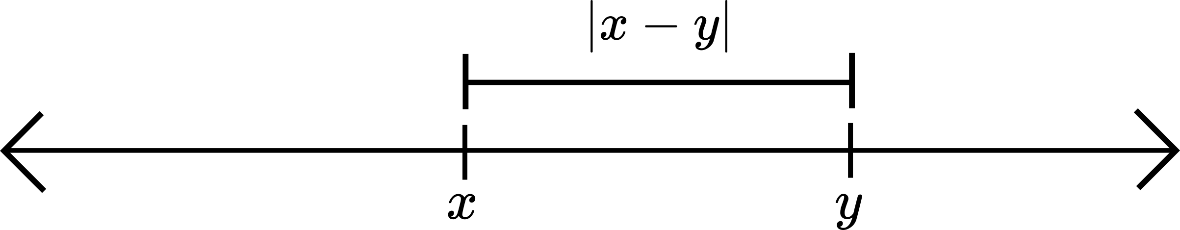
The absolute value gives us a notion of distance, in particular, we define the distance between two real numbers \(x\) and \(y\) to be the quantity \(|x-y|\).

One property that distance should satisfy is the following: Given three points \(a,b,\) and \(c\), the distance from \(a\) to \(c\) should not be greater than the distance from \(a\) to \(b\) plus the distance from \(b\) to \(c\). For this distance, this statement takes the following form:

\[|a-c|\leq |a-b|+|b-c|.\]

If we set \(x=a-b\) and \(y=b-c\), then \(a-c=x+y\), and the above inequality becomes

\[|x+y|\leq |x|+|y|.\]

This last inequality is called the triangle inequality.

Example. If \(x\) is a real number such that \(|x-4|<2\), then how large can \(|x+4|\) be?

Part 4:

Topology

(See sections 3.1-3.15 in Apostol)

Definition 3.1. Let \(n>0\) be an integer. An ordered set of \(n\) real numbers is called an \(n\)-tuple, a \(n\)-dimensional point or a vector with \(n\) components. Points will be denoted with bold-face letters, for example:

\[\mathbf{x} = (x_{1},x_{2},\ldots,x_{n}).\]

The number \(x_{k}\) above is called the \(k\)th coordinate of the point \(\mathbf{x}\). The set of all \(n\)-dimensional points is call \(n\)-dimensional Euclidean space, and is denoted by \(\mathbb{R}^{n}\).

Below are graphical depictions of \(\mathbb{R}^{1}=\mathbb{R}\) and \(\mathbb{R}^{2}\).

Definition 3.2. Let \(\mathbf{x} = (x_{1},x_{2},\ldots,x_{n})\) and \(\mathbf{y} = (y_{1},y_{2},\ldots,y_{n})\) be in \(\mathbb{R}^{n}\). We define

a) \(\mathbf{x} = \mathbf{y}\) if and only if \(x_{i}=y_{i}\) for all \(i=1,2,\ldots,n\).

b) \(\mathbf{x}+\mathbf{y} = (x_{1}+y_{1},x_{2}+y_{2},\ldots,x_{n}+y_{n})\)

c) For \(a\in\mathbb{R}\), \(a\mathbf{x} = (ax_{1},ax_{2},\ldots,ax_{n})\)

d) \(\mathbf{x}-\mathbf{y} = \mathbf{x}+(-1)\mathbf{y}\)

e) The zero vector or origin is the point

\[\mathbf{0} = (0,0,\ldots,0).\]

f) The inner product or dot product of \(\mathbf{x}\) and \(\mathbf{y}\) is the scalar:

\[\mathbf{x}\cdot\mathbf{y} = \sum_{k=1}^{n}x_{k}y_{k}.\]

g) The norm or length of a vector \(\mathbf{x}\) is the nonnegative number

\[\|\mathbf{x}\| = (\mathbf{x}\cdot\mathbf{x})^{1/2}.\]

The number \(\|\mathbf{x}-\mathbf{y}\|\) is the distance between \(\mathbf{x}\) and \(\mathbf{y}\). 

Length and distance in \(\mathbb{R}\) and \(\mathbb{R}^{2}\)

Theorem 3.3. Let \(\mathbf{x}\) and \(\mathbf{y}\) be points in \(\mathbb{R}^{n}\). Then,

a) \(\|\mathbf{x}\|\geq 0\), and \(\|\mathbf{x}\|=0\) if and only if \(\mathbf{x} = \mathbf{0}\).

b) \(\|a\mathbf{x}\| = |a|\|\mathbf{x}\|\) for all \(a\in\mathbb{R}.\)

c) \(\|\mathbf{x} - \mathbf{y}\| = \|\mathbf{y} - \mathbf{x}\|\)

d) (Cauchy-Schwarz inequality) \(|\mathbf{x}\cdot\mathbf{y}|\leq \|\mathbf{x}\|\|\mathbf{y}\|\)

e) (triangle inequality) \(\|\mathbf{x} +\mathbf{y}\| \leq \|\mathbf{x}\| + \|\mathbf{y}\|\)

Open sets and open balls

Let\(\mathbf{x}\) be a point in \(\mathbb{R}^{n}\). For \(r>0\) consider all the set of points in \(\mathbb{R}^{n}\) which are a distance \(<r\) away from \(\mathbf{x}\)

This set is called an open ball of radius \(r\) and center \(\mathbf{x}\), and is denoted

\[B(\mathbf{x};r)=\{\mathbf{y}\in\mathbb{R}^{n} : \|\mathbf{x}-\mathbf{y}\|<r\}.\]

In \(\mathbb{R}^{1}\), note that

\[B(x;r) = (x-r,x+r).\]

Definition 3.6. A set \(S\subset\mathbb{R}^{n}\) is called open if every point \(\mathbf{a}\in S\) is an interior point of \(S\). That is, \(S\) is open if for every \(\mathbf{a}\in S\) there exists a positive number \(r>0\) such that if \(\|\mathbf{a}-\mathbf{x}\|<r\), then \(\mathbf{x}\in S\). 

Definition 3.5. Let \(S\subset \mathbb{R}^{n}\). A point \(\mathbf{a}\in S\) is called an interior point of \(S\) if there exists \(r>0\) such that \(B(\mathbf{a};r)\subset S\).

An open set in \(\mathbb{R}^{2}:\)

Example. The set \(\{\mathbf{x}\in\mathbb{R}^{2} : \|\mathbf{x}\|\leq 1\}\) is not open:

Proposition 14. An open ball is an open set.

Proposition 15. Let \(\mathbf{x}\) and \(\mathbf{y}\) be points in \(\mathbb{R}^{n}\) and \(r,s>0\). If \(\|\mathbf{x}-\mathbf{y}\|<r+s\) then there exists \(\mathbf{z}\in\mathbb{R}^{n}\) and \(\delta>0\) such that \[B(\mathbf{z};\delta)\subset B(\mathbf{x};r)\cap B(\mathbf{y};s)\]

Proposition 15. Let \(\mathbf{x}\) and \(\mathbf{y}\) be points in \(\mathbb{R}^{n}\) and \(r,s>0\). If \(\|\mathbf{x}-\mathbf{y}\|<r+s\) then there exists \(\mathbf{z}\in\mathbb{R}^{n}\) and \(\delta>0\) such that \[B(\mathbf{z};\delta)\subset B(\mathbf{x};r)\cap B(\mathbf{y};s)\]

We can assume without loss of generality that \(r\geq s\), but what if \(r\gg s\) (\(r\) is much bigger than \(s\))?

Is our picture generic enough?

Proof continued.  Case 2. Suppose that \(r<  s+\|\mathbf{x}-\mathbf{y}\|.\)

Define

\[\delta = \frac{r+s-\|\mathbf{x} - \mathbf{y}\|}{2}\quad \text{and}\quad \mathbf{u} = \frac{\mathbf{y}-\mathbf{x}}{\|\mathbf{x}-\mathbf{y}\|}\quad\text{and}\quad\mathbf{z} = \mathbf{x}+(r-\delta)\mathbf{u}.\]

Since \(\|\mathbf{x}-\mathbf{y}\|<r+s\) we see that \(\delta>0\).

Let \(\mathbf{w}\in B(\mathbf{z};\delta)\), that is, \(\|\mathbf{z}-\mathbf{w}\|<\delta.\) We must show that \(\mathbf{w}\in B(\mathbf{x};r)\) and \(\mathbf{w}\in B(\mathbf{y};s).\) Note that since \(r\geq s\) we have

\[r-\delta = r-\frac{r+s-\|\mathbf{x} - \mathbf{y}\|}{2}=\frac{r-s+\|\mathbf{x} - \mathbf{y}\|}{2}\geq \frac{\|\mathbf{x} - \mathbf{y}\|}{2}\geq 0\]

Therefore,

\(\displaystyle{<\|-(r-\delta)\mathbf{u}\| +\delta = |-(r-\delta)|\|\mathbf{u}\| +\delta = r-\delta+\delta = r}\)

\(\|\mathbf{x}-\mathbf{w}\| = \|\mathbf{x}-\mathbf{z}+\mathbf{z}-\mathbf{w}\|\leq \|\mathbf{x}-\mathbf{z}\|+\|\mathbf{z}-\mathbf{w}\|\)

This shows that \(\mathbf{w}\in B(\mathbf{x};r).\)

Note that our assumtion that \(r< s+\|\mathbf{x}-\mathbf{y}\|\) is equivalent to \(s-r+\|\mathbf{x}-\mathbf{y}\|> 0.\) Thus, we have

\(\|\mathbf{y}-\mathbf{w}\| = \|\mathbf{y}-\mathbf{z}+\mathbf{z}-\mathbf{w}\|\leq \|\mathbf{y}-\mathbf{z}\|+\|\mathbf{z}-\mathbf{w}\|\)

\(\displaystyle{0<\frac{s-r+\|\mathbf{x}-\mathbf{y}\|}{2} = s-\delta.}\)

And, finally

\(\leq \|(s-\delta)\mathbf{u}\|+\|\mathbf{z}-\mathbf{w}\|<(s-\delta) + \delta = s.\)

This shows that \(\mathbf{w}\in B(\mathbf{y};s).\) \(\Box\)

Proof.  Note that

\[\mathbf{z} = \mathbf{x}+(r-\delta)\mathbf{u} = \mathbf{y}-(\mathbf{y}-\mathbf{x}) + \frac{r-\delta}{\|\mathbf{x}-\mathbf{y}\|}(\mathbf{y}-\mathbf{x})\]

\[=\mathbf{y} - \left(1-\frac{r-\delta}{\|\mathbf{x}-\mathbf{y}\|}\right)(\mathbf{y}-\mathbf{x}) = \mathbf{y} - \left(\|\mathbf{x}-\mathbf{y}\|-r+\delta\right)\mathbf{u}\]

\[= \mathbf{y}-(s-\delta)\mathbf{u}\]

Theorem 3.7. The union of any collection of open sets is open.

Theorem 3.8. The intersection of any finite collection of open sets is open.

Theorem 3.8. The intersection of any finite collection of open sets is open.

Example. For each \(n\in\mathbb{N}\) define the set

\[I_{n} = \left(-\frac{1}{n},1+\frac{1}{n}\right).\]

The intersection is

\[\bigcap_{n=1}^{\infty}I_{n} = [0,1]\]

which is not open.

Definition 3.12. A set \(S\subset\mathbb{R}^{n}\) is called closed if its complement \(\mathbb{R}\setminus S\) is open.

Note: The book uses the following notation for set complements: If \(X\) and \(Y\) are sets, then

\[X - Y = \{x\in X : x\notin Y\}.\]

We will often use the notation \(X\setminus Y\) for the same set.

Example. Given \(a\leq b\), the closed interval

\[[a,b]=\{x\in\mathbb{R} : a\leq x\leq b\}\]

is a closed set, since

\[\mathbb{R}\setminus[a,b] = (-\infty,a)\cup (b,\infty)\]

is the union of two open intervals.

Example. The set \(K=\{\mathbf{x}\in\mathbb{R}^{2} : \|\mathbf{x}\|\leq 1\}\) is closed:

Note that the complement of \(K\) is the set

\[\mathbb{R}^{2}\setminus K = \{\mathbf{x}\in\mathbb{R}^{2} : \|\mathbf{x}\|>1\}.\]

If \(\mathbf{z}\in\mathbb{R}^{2}\setminus K\), then we let \(\mathbb{r}\in(0,\|\mathbf{z}\|-1).\) It is straightforward to show that \(B(\mathbf{z};r)\subset \mathbb{R}^{2}\setminus K.\)

Example. The set \((0,1]\) is neither open nor closed.

Example. The set \(\mathbb{Q}\) is neither open nor closed.

Theorem 3.13. The union of a finite collection of closed sets is closed, and the intersection of any collection of closed sets is closed.

Theorem 3.13 follows from Theorems 3.7 and 3.8 and De Morgan's laws: Given a collection of sets \(\{A_{x}\}_{x\in X}\) which are all subsets of \(\mathbb{A}\) we have

\[\mathbb{A}\setminus\bigcup_{x\in X}A_{x} = \bigcap_{x\in X}(\mathbb{A}\setminus A_{x})\]

and

\[\mathbb{A}\setminus\bigcap_{x\in X}A_{x} = \bigcup_{x\in X}(\mathbb{A}\setminus A_{x})\]

Theorem 3.14. If \(A\) is open and \(B\) is closed, the \(A\setminus B\) is open, and \(B\setminus A\) is closed.

Proof. Observe that

\[A\setminus B = A\cap (\mathbb{R}^{n}\setminus B)\]

Hence, by De Morgan's law

\[\mathbb{R}^{n}\setminus(A\setminus B) = (\mathbb{R}^{n}\setminus A)\cup B.\]

This is the union of two closed sets, and hence closed. This shows that \(A\setminus B\) is open.

The other proof is similar. (You should try it!) \(\Box\)

Definition 3.15. Let \(S\subset \mathbb{R}^{n}\) and \(\mathbf{x}\in\mathbb{R}^{n}\). The point \(\mathbf{x}\) is called an adherent point of \(S\) if every open ball \(B(\mathbf{x};r)\) contains at least one point of \(S\). That is, for every \(r>0\) there exists a point \(\mathbf{z}\in B(\mathbf{x};r)\cap S\).

Example.  Consider the set \(S=(0,1]\cup\{2\}\). As we already noted, every point of \(S\) is an adherent point of \(S\). Note that \(0\notin S\), but \(0\) is an adherent point of \(S\). The set \(S\) has no other adherent points. Thus, the set of adherent points of \(S\) is \([0,1]\cup\{2\}\).

Example.  Consider the set 

\[T = \left\{\frac{1}{n} : n\in\N\right\}\]

The set of adherent points of \(T\) is the set \(T\cup\{0\}\).

Observe that given \(S\subset\mathbb{R}^{n}\), every point in \(S\) is an adherent point of \(S\).

Example.  Consider the set \(\mathbb{Q}\). The set of adherent points of \(\mathbb{Q}\) is \(\mathbb{R}\).

Definition 3.16. Let \(S\subset \mathbb{R}^{n}\) and \(\mathbf{x}\in\mathbb{R}^{n}\). The point \(\mathbf{x}\) is called an accumulation point of \(S\) if every open ball \(B(\mathbf{x};r)\) contains at least one point of \(S\) distinct from \(\mathbf{x}\). That is, for every \(r>0\) there exists a point \(\mathbf{z}\in (B(\mathbf{x};r)\setminus\{\mathbf{x}\})\cap S\).

Example.  Consider the set \(S=(0,1]\cup\{2\}\). The set of accumulation points of \(S\) is \([0,1]\).

Example.  Consider the set 

\[T = \left\{\frac{1}{n} : n\in\N\right\}\]

The set of accumulation points of \(T\) is the set \(\{0\}\).

Observe that given \(S\subset\mathbb{R}^{n}\), points in \(S\) may or may not be accumulation points of \(S\). Points of \(S\) which are not accumulation points of \(S\) are called isolated points of \(S\).

Example.  Consider the set \(\mathbb{Q}\). The set of accumulation points of \(\mathbb{Q}\) is \(\mathbb{R}\).

Theorem 3.17. If \(\mathbf{x}\) is an accumulation point of \(S\), then every ball \(B(\mathbf{x};r)\) contains infinitely many points of \(S\).

Proof. On the board and in the book.

Definition 3.19. The set of all adherent points of a set \(S\) is called the closure of \(S\) and is denoted by \(\overline{S}\).

Theorem 3.18, 3.20 & 3.22. Given \(S\subset\mathbb{R}^{n}\), the following are equivalent:

1. \(S\) is closed.
2. \(S\) contains all of its adherent points, that is, \(\overline{S}\subset S\)
3. \(S = \overline{S}\).
4. \(S\) contains all of its accumulation points.

Proof. On the board and in the book.

Definition 3.23. A set \(S\subset\mathbb{R}^{n}\) is said to be bounded if there exists \(r>0\) and \(\mathbf{x}\in\mathbb{R}^{n}\) such that \(S\subset B(\mathbf{x};r).\)

Examples:

• Any open ball is bounded.
• The set of natural numbers \(\mathbb{N}\subset\mathbb{R}\) is not bounded
• The set of integers \(\mathbb{Z}\subset\mathbb{R}\) is not bounded.
• The whole space \(\mathbb{R}^{n}\) is not bounded.
• Any finite set is bounded:

Proof. If \(X=\{\mathbf{x}_{1},\mathbf{x}_{2},\ldots,\mathbf{x}_{N}\}\subset\mathbb{R}^{n}\), then let

\[r =1+\max \{\|\mathbf{x}_{1}\|,\|\mathbf{x}_{2}\|,\ldots,\|\mathbf{x}_{N}\|\}.\] Then, for each \(i\in\{1,2,\ldots,n\}\) we observe that

\[\|\mathbf{0}-\mathbf{x}_{i}\| = \|\mathbf{x}_{i}\|\leq \max \{\|\mathbf{x}_{1}\|,\|\mathbf{x}_{2}\|,\ldots,\|\mathbf{x}_{N}\|\}<r\]

and hence \(X\subset B(\mathbf{0};r)\). \(\Box\)

Theorem 3.24 (Bolzano-Weierstrass). If \(S\subset\mathbb{R}^{n}\) is bounded and infinite, then there is at least one point of \(\mathbb{R}^{n}\) which is an accumulation point of \(S\).

Proof. On the board and in the text.

Notes:

• The set \(S\) need not contain any accumulation points: \[S=\left\{\frac{1}{n} : n\in\mathbb{N}\right\}\] has only one accumulation point, namely, \(0\), but \(0\notin S\).
• The assumption that \(S\) is bounded is necessary. The set of integers \(\mathbb{Z}\) is infinte, but not bounded, and no point in \(\mathbb{R}\) is an accumulation point of \(\mathbb{Z}\)

Theorem 3.25 (Cantor intersection theorem). Let \(\{Q_{1},Q_{2},\ldots\}\) be a countable collection of nonempty sets in \(\mathbb{R}^{n}\) such that

  i) \(Q_{k+1}\subset Q_{k}\) for each \(k\in\mathbb{N}\)

  ii) \(Q_{k}\) is closed and bounded for each \(k\in\mathbb{N}\).

Then, the intersection \[\bigcap_{k=1}^{\infty}Q_{k}\] is closed and nonempty.

Note: The assumptions that the \(Q_{k}\)'s are both closed and bounded are both necessary:

The sets \(Q_{k} = [k,\infty)\) are closed, but not bounded, and \[\bigcap_{k=1}^{\infty}[k,\infty)=\varnothing\]

The sets \(Q_{k} = (0,\frac{1}{k})\) are bounded but not closed, and\[\bigcap_{k=1}^{\infty}\left(0,\tfrac{1}{k}\right) = \varnothing\]

Proof. Set

\[Q = \bigcap_{k=1}^{\infty}Q_{k}.\]

Since each of the sets \(Q_{k}\) is closed, the intersection is closed by Theorem 3.13.

For each \(k\in\mathbb{N}\) let \(\mathbf{a}_{k}\in Q_{k}\) and set

\[A: = \{\mathbf{a}_{1},\mathbf{a}_{2},\ldots\}.\]

If \(A\) is finite, then there exists \(\mathbf{a}\in A\) such that \(\mathbf{a}_{k}=\mathbf{a}\) for infinitely many \(k\in\N\). Thus, if \(j\in\N\), there exists \(k\geq j\) such that \[\mathbf{a}=\mathbf{a}_{k}\in Q_{k}\subset Q_{k-1}\subset\cdots\subset Q_{j}.\]

This shows that \(\mathbf{a}\in Q_{j}\) for each \(j\in\N\), and thus \(\mathbf{a}\in Q\).

Now, we may assume \(A\) is an infinite set. Since \(Q_{k}\subset Q_{1}\) for all \(k\in\N\) we see that \(\mathbf{a}_{k}\in Q_{1}\) for each \(k\in\N\), and thus \(A\subset Q_{1}\). Since \(Q_{1}\) is bounded, this implies \(A\) is bounded.

Proof continued. By the Bolzano-Weierstrass theorem the set \(A\) has an accumulation point, call it \(\mathbf{a}\).

By Theorem 3.17, every open ball around \(\mathbf{a}\) contains infinitely many points of \(A\).

Let \(k\in\N\) be arbitrary, and note that \[\{\mathbf{a}_{k},\mathbf{a}_{k+1},\ldots\}\subset Q_{k}.\]

From this we deduce that every open ball around \(\mathbf{a}\) also contains infinitely many points of \(Q_{k}\). This implies that \(\mathbf{a}\) is an accumulation point of \(Q_{k}\), and since \(Q_{k}\) is closed, we see that \(\mathbf{a}\in Q_{k}\). Since \(k\in\N\) was arbitrary, we conclude that \(\mathbf{a}\in Q_{k}\) for all \(k\in\N\), and thus \[\mathbf{a}\in \bigcap_{k=1}^{\infty}Q_{k}.\]

\(\Box\)

Definition 3.26. Given a set \(S\subset\mathbb{R}^{n}\), a collection of sets \(F\) is called a covering of \(S\) if

\[S\subset \bigcup_{A\in F}A.\]

If \(F\) is a covering of \(S\) and each set in \(F\) is an open set, then \(F\) is called an open covering (or open cover) of \(S\).

Examples.

1. The collection \[F=\{(0.9,1.1),(1.9,2.1),\ldots,(k-\tfrac{1}{10},k+\tfrac{1}{10}),\ldots\}\] is an open cover of \(\mathbb{N}\).
2. For each rational number \(q\in\mathbb{Q}\) select a positive number \(r_{q}>0\). Then, the set \[F = \{(q-r_{q},q+r_{q}):q\in\mathbb{Q}\}\] is an open cover of \(\mathbb{Q}\).
3. More generally, if \(S\subset\mathbb{R}^{n}\), then for each \(\mathbf{x}\in S\) select a positive number \(r_{\mathbf{x}}>0\), then the set \(F=\{B(\mathbf{x};r_{\mathbf{x}}) : \mathbf{x}\in S\}\) is an open cover of \(S\).

Definition 3.30. A set \(S\subset\mathbb{R}^{n}\) is said to be compact if every open cover of \(S\) contains a finite subcover, that is, if \(F\) is an open cover of \(S\), then there is a finite subset of \(F\) which is also a cover of \(S\).

Proposition 16. For \(a\leq b\), the set \([a,b]\subset\mathbb{R}\) is compact.

Proof. If \(a=b\), then \([a,b]=\{a\}\). It is clear that any open cover of a \(\{a\}\) has a finite subcover, so we will now suppose that \(a<b\).

Suppose that \(F\) is an open cover of \([a,b]\). Since \[a\in\bigcup_{U\in F}U,\]

there is an open set \(U\in F\) such that \(a\in U\). Since \(U\) is open, there exists \(r>0\) such that \(B(a;r)\subset U\). Thus, \([a,a+\frac{r}{2}]\subset U\). Define the set

\[A=\{s\in[a,b] : \text{a finite subset of \(F\) covers } [a,s]\}.\]

We have already seen that \(a+\frac{r}{2}\in A\), so \(A\neq \varnothing\), and by definition \(A\) is bounded above, so we set

\[c = \sup A.\]

Proof continued.

Case 1. Suppose \(c=b\). There exists \(V\in F\) such that \(b\in V\). Since \(V\) is open, there exists \(\varepsilon>0\) such that \((b-\varepsilon,b+\varepsilon)\subset V\). Since \(b=\sup A\), we deduce that \([a,b-\varepsilon]\) can be covered by a finite subset of \(X\subset F\). Thus \(X\cup \{V\}\) is a finite subset of \(F\) that covers \([a,b]\).

Case 2. Suppose \(c<b\). There exists \(W\in F\) such that \(c\in W\) since \(W\) is open, there exists \(\delta>0\) such that \((c-\delta,c+\delta)\subset W\). Since \(c-\delta<c\) there exists \(d>c-\delta\) such that \([a,d]\) can be covered by a finite subset \(Y\subset F\). Then \(Y\cup \{W\}\) is an open cover of \([a,c+\frac{\delta}{2}]\). This contradiction shows that \(c=b\), that is, we are reduced to Case 1 where we have already seen that the desired conclusion holds. \(\Box\)

Theorem 3.29 (the Heine-Borel theorem). A set \(S\subset \mathbb{R}^{n}\) is compact if and only if it is closed and bounded.

Proposition 17. If \(K\subset\mathbb{R}^{n}\) is compact and \(L\subset K\) is closed, then \(L\) is compact.

Proof. Let \(F\) be an open cover of \(L\). The set \(F_{1} = F\cup\{\mathbb{R}^{n}\setminus L\}\) is an open cover of \(K\). By definition, there is a finite subset \(G\subset F_{1}\) that covers \(K\), and hence also covers \(L\). The set \(G\) might contain \(\mathbb{R}^{n}\setminus L\), but the rest of \(G\) is still a finite subcover that covers \(L\). \(\Box\)

Proof sketch. Using Proposition 16 and induction we can show that for any \(a\geq 0\), the set \([-a,a]^{n}\) is compact in \(\mathbb{R}^{n}\).

Since \(S\) is bounded, there exists \(a>0\) such that \(S\subset[-a,a]^{n}\).

The theorem follows from Proposition 17. \(\Box\)

Metric spaces

Definition 3.32. A metric space is a nonempty set \(M\) (the elements of this set are called points) and a function \(d:M\times M\to\mathbb{R}\) (called a metric) such that for any \(x,y,z\in M\) the following four properties hold:

  1. \(d(x,x)=0\)

  2. \(d(x,y)>0\) for \(x\neq y\)

  3. \(d(x,y)=d(y,x)\)

  4. \(d(x,y)\leq d(x,z)+d(z,y).\)

When we want to be clear, we denote a metric space as a pair \((M,d).\)

Examples.

1) The most important example of a metric space is \(\mathbb{R}^{n}\) with

\[d(\mathbf{x},\mathbf{y}) = \|\mathbf{x}-\mathbf{y}\|.\]

2) Consider the set \(\mathbb{Q}\) with \(d(x,y)=|x-y|\), this is also a metric space. More generally, any subset \(M\subset \mathbb{R}^{n}\) with metric \(d(\mathbf{x},\mathbf{y}) = \|\mathbf{x}-\mathbf{y}\|\) is a metric space.

More examples. An example of a metric space often worth considering is the set \([0,1]\subset \mathbb{R}\) together with the metric \(d(x,y)=|x-y|\).

There are other metrics that can be defined on \(\mathbb{R}^{n}\). Given

\(\mathbf{x} = (x_{1},x_{2},\ldots,x_{n})\) and \(\mathbf{y} = (y_{1},y_{2},\ldots,y_{n})\) in \(\mathbb{R}^{n}\) the following functions are metrics on \(\mathbb{R}^{n}\):

\[d(\mathbf{x},\mathbf{y}) = \sum_{i=1}^{n}|x_{i}-y_{i}|,\]

\[d(\mathbf{x},\mathbf{y}) = \max\{|x_{1}-y_{1}|,|x_{2}-y_{2}|,\ldots,|x_{n}-y_{n}|\},\]

for any \(p\geq 1\)

\[d(\mathbf{x},\mathbf{y})=\left(\sum_{i=1}^{n}|x_{i}-y_{i}|^{p}\right)^{1/p}.\]

Part 5:

Limits and continuity

(See sections 4.1-4.5, 4.7-4.9, 4.11-4.15  in Apostol)

Functions

Definition. Given two sets \(X\) and \(Y\), a subset

\[F\subset X\times Y=\{(x,y) : x\in X,\ y\in Y\}\]

is called a function if it satisfies the following two properties:

1. for each \(x\in X\) there exists \(y\in Y\) such that \((x,y)\in F\)
2. if \((x,y)\in F\) and \((x,z)\in F\), then \(y=z\).

Some more function terminology:

• The set \(X\) is called the domain of \(F\).
• The set \(Y\) is called the codomain of \(F\).
• The inclusion \((x,y)\in F\) is written \(F(x) = y\), and read "\(F\) of \(x\) equals \(y\)."
• The set \[\operatorname{im}(F) = \{F(x) : x\in X\}\] is called the range or image of \(F\).
• To denote \(F\) is a function with domain \(X\) and codomain \(Y\) we write \(F:X\to Y\).

• The elements of the domain \(X\) are sometimes called inputs and the elements of the range \(\operatorname{im}(F)\) are called outputs.
• The set of all functions with domain \(X\) and codomain \(Y\) is sometimes denoted \(Y^{X}\).
• A function \(F:X\to Y\) is called onto or a surjection if \(\operatorname{im}(F)=Y\).
• A function \(F:X\to Y\) is called one-to-one or an injection if \(F(x)=F(y)\) implies \(x=y\).

Defining a function:

The most common way to define a function is by a rule:

Let \(f:\mathbb{R}\to \mathbb{R}\) be given by \(f(x) = x^{2}\) for all \(x\in\mathbb{R}\).

Another example of a rule, is a so-called piecewise definition:

Let \(g:(-\infty,0)\cup(0,\infty)\to\mathbb{R}\) be given by \(g(x) = \begin{cases} \frac{1}{x} & x>0,\\ \frac{-1}{x} & x<0.\end{cases}\)

More on defining functions:

If the domain of a function is finite, then we can simply specify each output for a given input:

Let \(h:\{1,2,3\}\to\mathbb{R}\) be given by

\[h(1)=-3,\ h(2) = \pi,\ h(3)=0.\]

Showing that two functions are equal:

Suppose that we have two functions \(f:X\to Y\) and \(g:X\to Y\)

What does it mean to say that \(f=g\)?

For each \(x\in X\), \(f(x) = g(x)\).

A function is a special type of set, it is not an equation.

Sequences

Definition. Let \(X\) be a set. A sequence in \(X\) is a function \(x:\mathbb{N}\to X\).

Definition 4.1. A sequence \(\{x_{n}\}\) of points in a metric space \((S,d)\) is said to converge if there is a point \(p\in S\) with the following property:

For every \(\varepsilon>0\) there exists \(N\in\mathbb{N}\) such that \[d(x_{n},p)<\varepsilon\quad\text{for all }n\geq N.\]

In this case we say that \(\{x_{n}\}\) converges to \(p\), and we write \(x_{n}\to p\) as \(n\to\infty\), or just \(x_{n}\to p\). If there is no such \(p\in S\), then we say that \(\{x_{n}\}\) diverges or does not converge.

For sequence \(x:\mathbb{N}\to X\) we write \(x_{n}\) instead of \(x(n)\), and the function is denoted \(\{x_{n}\}\), or \(\{x_{n}\}_{n=1}^{\infty}\). 

For example, we could define a sequence in \(\mathbb{R}\) by saying the following:

Let \(\{x_{n}\}\) be given by \(x_{n} = \dfrac{n}{n+1}\quad\text{for each }n\in\mathbb{N}.\)

Proposition. The sequence \(\{\frac{1}{n}\}\) converges to \(0\).

Proof. Let \(\varepsilon>0\) be given. Fix \(N\in\N\) such that \(N>\frac{1}{\varepsilon}.\) For \(n\geq N\), we see that \(n>\frac{1}{\varepsilon}\), and thus

\[\left|\frac{1}{n}-0\right| = \frac{1}{n}<\varepsilon.\]

\(\Box\)

Proposition.   \(\displaystyle{\frac{n}{2n+1}\to\frac{1}{2}}\).

Proposition.   \(\displaystyle{\frac{2n^{2}+n+1}{n^2+1}\to 2}\).

Scratch work. We wish to show that

\[\left|\frac{2n^2+n+1}{n^2+1}-2\right|<\varepsilon.\]

So, we simplify this inequality as follows:

\[\varepsilon>\left|\frac{2n^2+n+1}{n^2+1}-2\right| = \left|\frac{n-1}{n^{2}+1}\right| = \frac{n-1}{n^{2}+1},\]

and hence we want

\[\frac{n-1}{n^{2}+1}<\varepsilon.\]

Instead, let's look for a sequence \(\{x_{n}\}\) which more obviously converging to zero, but such that

\[\frac{n-1}{n^{2}+1}<\quad \]

Proposition.   \(\displaystyle{\frac{2n^{2}+n+1}{n^2+1}\to 2}\).

Proof. Let \(\varepsilon>0\) be given. Choose \(N\in\N\) such that \(N>\frac{1}{\varepsilon}\). Let \(n\geq N\). We first observe that \[\frac{1}{n}\leq\frac{1}{N}<\varepsilon.\]

Next, we obvserve that

\[\left|\frac{2n^{2}+n+1}{n^{2}+1}-2\right| = \left|\frac{n-1}{n^{2}+1}\right| = \frac{n-1}{n^{2}+1}<\frac{n}{n^{2}} = \frac{1}{n}<\varepsilon.\]

\(\Box\)

Proposition.   \(\displaystyle{\frac{n^2+n-1}{n^2-2}\to 1}\).

Scratch work. We wish to show that

\[\left|\frac{n^2+n-1}{n^2-2}-1\right|<\varepsilon.\]

So, we simplify this inequality as follows:

\[\varepsilon>\left|\frac{n^2+n-1}{n^2-2}-1\right| = \left|\frac{n+1}{n^{2}-2}\right|\]

For \(n\geq 2\) we see that \(\dfrac{n+1}{n^{2}-2}>0\), and hence we want

\[\frac{n+1}{n^{2}-2}<\varepsilon.\]

Again, we look for a sequence which is bigger, but more obviously converging to zero:

\[\frac{n+1}{n^{2}-2}\leq\frac{n+n}{n^{2}-2} = \frac{2n}{n^{2}-2}\leq\frac{2n}{n^{2}-n} = \frac{2}{n-1}\]

Proposition.   \(\displaystyle{\frac{n^2+n-1}{n^2-2}\to 1}\).

Proof. Let \(\varepsilon>0\) be given. Choose \(N\in\N\) such that 

\[N>1+\frac{2}{\varepsilon}.\]

This implies

\[\frac{2}{N-1}<\varepsilon.\]

If \(n\geq N\) then we see that

\[\frac{2}{n-1}\leq\frac{2}{N-1}<\varepsilon.\]

Since \(N>1\) and \(N\in\N\), we deduce that \(n\geq 2\). Finally, we have

\[\left|\frac{n^2+n-1}{n^2-2}-1\right| = \frac{n+1}{n^{2}-2}\leq \frac{n+n}{n^{2}-2} = \frac{2n}{n^{2}-2}\leq \frac{2n}{n^{2}-n} = \frac{2}{n-1}<\varepsilon.\]

\(\Box\)

Proposition. Let \(\{\mathbf{x}_{n}\}\) and \(\{\mathbf{y}_{n}\}\) be sequences in \(\mathbb{R}^{n}\). If \(\mathbf{x}_{n}\to \mathbf{a}\) and \(\mathbf{y}_{n}\to\mathbf{b}\), then \(\mathbf{x}_{n}+\mathbf{y}_{n}\to \mathbf{a}+\mathbf{b}\).

Proof. Let \(\varepsilon>0\) be given. There exists \(N_{1}\in\mathbb{N}\) such that

\[\|\mathbf{x}_{n}-\mathbf{a}\|<\frac{\varepsilon}{4}\quad\text{for all }n\geq N_{1},\]

and there exists \(N_{2}\in\mathbb{N}\) such that

\[\|\mathbf{y}_{n}-\mathbf{b}\|<\frac{\varepsilon}{4}\quad\text{for all }n\geq N_{2}.\]

Let \(N=\max\{N_{1},N_{2}\}\) and let \(n\geq N\) be arbitrary. This implies \(n\geq N_{1}\) and \(n\geq N_{2}\), and thus

\[\|(\mathbf{x}_{n} +\mathbf{y}_{n}) - (\mathbf{a}+\mathbf{b})\| = \|\mathbf{x}_{n} - \mathbf{a} +\mathbf{y}_{n}-\mathbf{b}\| \leq \|\mathbf{x}_{n} - \mathbf{a}\| +\|\mathbf{y}_{n}-\mathbf{b}\|\]

\[<\frac{\varepsilon}{4}+\frac{\varepsilon}{4} = \frac{\varepsilon}{2}<\varepsilon.\]

\(\Box\)

Proposition. Let \(\{x_{n}\}\) and \(\{y_{n}\}\) be sequences in \(\mathbb{R}\). If \(x_{n}\to a\) and \(y_{n}\to b\), then \(x_{n}y_{n}\to ab\).

First presentation:

Hints:

• First show that there is some \(M\) such that \(|x_{n}|\leq M\) for all \(n\in\N\). 
• Use the fact that for any \(n\in\N\) \[x_{n}y_{n} - ab = x_{n}y_{n}-x_{n}b+x_{n}b-ab = x_{n}(y_{n}-b)+(x_{n}-a)b.\]

Definition. Let \(\{x_{n}\}\) be a sequence in a metric space \((S,d)\), and let \(\{n_{k}\}\) a strictly increasing sequence of natural numbers, that is, \(n_{k}\in\N\) for each \(k\in\N\), and 

\[n_{1}<n_{2}<n_{3}<\cdots<n_{k}<\cdots.\]

The sequence \(\{x_{n_{k}}\}_{k=1}^{\infty}\) is called a subsequence of \(\{x_{n}\}\). 

Subsequences

Definition 4.7. A sequence \(\{x_{n}\}\) in a metric space \((S,d)\) is called a Cauchy sequence if for every \(\varepsilon>0\) there exists \(N\in\N\) such that

\[d(x_{n},x_{m})<\varepsilon\quad\text{for all }m\geq N\text{ and }n\geq N.\]

Cauchy Sequences

Limits of functions

Definition 4.11. If \(p\) is an accumulation point of \(A\) and \(b\in T\), then 

\[\lim_{x\to p}f(x) = b\]

is defined to mean the following: For every \(\varepsilon>0\), there exists \(\delta>0\) such that

\[d_{T}(f(x),b)<\varepsilon\quad\text{for all }x\in (B(p;\delta)\setminus \{p\})\cap A.\]

In this case, we say that "\(b\) is the limit of \(f(x)\) as \(x\) tends to \(p\)."

Suppose \((S,d_{S})\) and \((T,d_{T})\) are metric spaces, and \(A\subset S\). Let \(f:A\to T\) be a function with domain \(A\) and codomain \(T\).

For example, we could have \(S=\mathbb{R}^{2}\) and \(T=\mathbb{R}\) with their usual metrics. Then we define the function \(f: B(\mathbf{0};1)\to\mathbb{R}\) by setting

\[f(x,y) = \frac{1-x^2}{1-x^{2}-y^{2}}\quad\text{for all }(x,y)\in B(\mathbf{0};1).\]

For every \(\varepsilon>0\) there exists \(\delta>0\) such that

\[\text{if }0<|x-p|<\delta,\text{ then }|f(x) - b|<\varepsilon\]

\(f:\mathbb{R}\to\mathbb{R}\)

For every \(\varepsilon>0\) there exists \(\delta>0\) such that

\[\text{if }0<\|x-p\|<\delta,\text{ then }\|f(x) - b\|<\varepsilon\]

\(f:\mathbb{R}^{n}\to\mathbb{R}^{m}\)

For every \(\varepsilon>0\) there exists \(\delta>0\) such that

\[\text{if }0<|x-p|<\delta\text{ and }x\in[a,b],\text{ then }|f(x) - b|<\varepsilon\]

\(f:[a,b]\to\mathbb{R}\)

\[\lim_{x\to p}f(x) = b\]

Proposition. \(\displaystyle{\lim_{x\to 0}x = 0}.\)

Scratch work. Suppose \(\varepsilon>0\). We wish to find \(\delta>0\) such that if \[0<|x-0|<\delta,\] then \[|x-0|<\varepsilon.\]  We should take \(\delta=\varepsilon\).

Proof. Let \(\varepsilon>0\) be given. Set \(\delta=\varepsilon\). For \(x\in\mathbb{R}\) such that \(|x-0|<\delta\), it is clear that \(|x-0|<\varepsilon.\) \(\Box\)

Proposition. \(\displaystyle{\lim_{x\to 0}x^2 = 0}.\)

Scratch work. Suppose \(\varepsilon>0\). We wish to find \(\delta>0\) such that if \[0<|x-0|<\delta,\] then \[|x^2-0|<\varepsilon.\] Since \(|x^{2}|=x^{2}\) it is enough to take \(\delta=\sqrt{\varepsilon}\).

Proof. Let \(\varepsilon>0\) be given. Set \(\delta=\sqrt{\varepsilon}\). For \(x\in\mathbb{R}\) such that \(|x-0|<\delta\), we see that

\[|x^{2} - 0| = |x|^{2}<\delta^{2} = \varepsilon.\ \Box\]

Proposition. For \(a\in\mathbb{R}\), \(\displaystyle{\lim_{x\to a}x^2 = a^2}.\)

Scratch work. Suppose \(\varepsilon>0\). We wish to find \(\delta>0\) such that if \[0<|x-a|<\delta,\] then \[|x^2-a^2|<\varepsilon.\] We can simplify the expression that we are trying to bound:

\[|x^{2}-a^{2}| = |x-a||x+a|.\]

As long as \(|x-a|<1\), which we can guarantee by choosing \(\delta\leq 1\), then by the triangle inequality \[|x+a|\leq |x-a|+|2a|<1+2|a|.\]

Thus, it should be enough to take \[\delta=\min\left\{1,\frac{\varepsilon}{1+2|a|}\right\}.\]

Proposition. For \(a\in\mathbb{R}\), \(\displaystyle{\lim_{x\to a}x^2 = a^2}.\)

Proof. Let \(\varepsilon>0\) be given. Set \[\delta=\min\left\{1,\frac{\varepsilon}{1+2|a|}\right\}.\]

Let \(|x-a|<\delta\). Since \(\delta\leq 1\), by the triangle inequality

\[|x+a|\leq |x-a|+|2a|<\delta+|2a|\leq 1+2|a|.\]

Since \(\delta\leq \frac{\varepsilon}{1+2|a|}\) we have

\[|x^{2}-a^{2}| = |x-a||x+a|\leq \frac{\varepsilon}{1+2|a|}|x+a|<\frac{\varepsilon}{1+2|a|}(1+2|a|) = \varepsilon. \ \Box\]

Proposition. For \(a\in\mathbb{R}\setminus\{0\}\), \(\displaystyle{\lim_{x\to a}\dfrac{1}{x} = \dfrac{1}{a}}.\)

Proof. Let \(\varepsilon>0\) be given. Set

\[\delta = \min\left\{\frac{1}{2}|a|,\frac{a^{2}\varepsilon}{4}\right\}.\]

Take \(x\in\mathbb{R}\setminus\{0\}\) such that \(0<|x-a|<\delta.\) By the reverse triangle inequality, we have

\[|x|\geq |a| - |x-a|>|a|-\delta\geq |a| - \frac{1}{2}|a| = \frac{1}{2}|a|.\]

Using this, we have

\[\left|\frac{1}{x}-\frac{1}{a}\right| = \frac{|x-a|}{|a||x|}<\frac{|x-a|}{|a|\frac{1}{2}|a|} = \frac{2}{a^{2}}|x-a| < \frac{2}{a^{2}}\delta\leq \frac{2}{a^{2}}\frac{a^{2}\varepsilon}{4} = \frac{\varepsilon}{2}<\varepsilon.\ \Box\]

Theorem 4.12. Using the notation from Definition 4.11, If \(p\) is an accumulation point of \(A\) and \(b\in T\), then

\[\lim_{x\to p}f(x) = b\]

if and only if the sequence \(\{f(x_{n})\}\) converges to \(b\) for every sequence \(\{x_{n}\}\) in \(A\setminus\{p\}\) which converges to \(p\).

Theorem 4.14. If

\[\lim_{x\to p}f(x) = \mathbf{a}\quad\text{and}\quad\lim_{x\to p}g(x) = \mathbf{b},\]

then 

a) \(\displaystyle{\lim_{x\to p}[f(x)+g(x)] = \mathbf{a}+\mathbf{b}}\)

b) \(\displaystyle{\lim_{x\to p}\lambda f(x) = \lambda\mathbf{a}}\) for any scalar \(\lambda\).

Now, suppose that \(T=\mathbb{R}^{k}\) with the usual metric. (Of particular interest is the case of \(k=1\).)

c) \(\displaystyle{\lim_{x\to p}f(x)\cdot g(x) = \mathbf{a}\cdot\mathbf{b}}\)

d) \(\displaystyle{\lim_{x\to p}\|f(x)\| = \|\mathbf{a}\|}\).

Proposition. Let \(A\subset \R^{k}\), and let \(f,g:A\to\mathbb{R}^{n}.\) If \[\lim_{x\to p}f(x) = \mathbf{a}\quad\text{and}\quad\lim_{x\to p}g(x) = \mathbf{b},\]

then \[\lim_{x\to p}f(x)\cdot g(x) = \mathbf{a}\cdot\mathbf{b}.\]

Second presentation:

Hints: \(\bullet\) First, suppose \(A=S=\mathbb{R}\) with the usual metric and \(n=1\). The proof in this case will be quite similar to the first presentation, namely, you should use the following observations:

\[|f(x)g(x) - ab| = |f(x)g(x) - f(x)b+f(x)b-ab|\]

\[\leq |f(x)g(x)-f(x)b|+|f(x)b-ab|\]

\[= |f(x)||g(x)-b|+|b||f(x)-a|\]

• Show that for some \(r>0\) the set \(\{f(x): x\in B(p;r)\setminus\{p\}\}\) is bounded.

Continuous Functions

Definition 4.15. A function \(f:S\to T\), where \(S\) and \(T\) are metric spaces is said to be continuous at a point \(p\) in \(S\) if for every \(\varepsilon>0\) there exists \(\delta>0\) such that

\[d_{T}(f(x),f(p))<\varepsilon\quad\text{for all }x\text{ satifying }d_{S}(x,p)<\delta.\]

If \(f\) is continuous at all \(p\) in some set \(A\subset S\), then we say that \(f\) is continuous on \(A\).

Definition 4.15 (For functions from \(\mathbb{R}^{m}\to\mathbb{R}^{k}\)). A function \(f:\mathbb{R}^{m}\to \mathbb{R}^{k}\) is said to be continuous at a point \(\mathbf{p}\) in \(\mathbb{R}^{m}\) if for every \(\varepsilon>0\) there exists \(\delta>0\) such that

\[\|f(\mathbf{x})-f(\mathbf{p})\|<\varepsilon\quad\text{for all }\mathbf{x}\text{ satifying }\|\mathbf{x}-\mathbf{p}\|<\delta.\]

Definition 4.15 (For functions from \(\mathbb{R}\to\mathbb{R}\)). A function \(f:\mathbb{R}\to \mathbb{R}\) is said to be continuous at a point \(p\) in \(\mathbb{R}\) if for every \(\varepsilon>0\) there exists \(\delta>0\) such that

\[|f(x)-f(p)|<\varepsilon\quad\text{for all }x \text{ satifying }|x-p|<\delta.\]

Proposition. For any \(p\in\mathbb{R}\), the function \(f:\mathbb{R}\to\mathbb{R}\) given by \(f(x) = x\) is continuous at \(p\). Thus \(f\) is continuous on \(\mathbb{R}\).

Proof. Let \(p\in\mathbb{R}\) and \(\varepsilon>0\) be given. Set \(\delta=\varepsilon\), and let \(x\in(p-\delta,p+\delta)\). Observe that \[|f(x) - f(p)| = |x-p|<\delta = \varepsilon.\ \Box\]

Proposition. For any \(p\in\mathbb{R}\), the function \(f:\mathbb{R}\to\mathbb{R}\) given by \(f(x) = 1\) is continuous at \(p\). Thus \(f\) is continuous on \(\mathbb{R}\).

Proof. Let \(p\in\mathbb{R}\) and \(\varepsilon>0\) be given. Set \(\delta=1\), then for any                   \(x\in(p-\delta,p+\delta)\) we have

\[|f(x) - f(p)| = |1-1|=0<\varepsilon.\ \Box\]

Corollary. Let \(a_{0},a_{1},\ldots,a_{n}\) be real numbers. Define the function \(f:\mathbb{R}\to\mathbb{R}\) by

\[f(x) = a_{0}+a_{1}x+a_{2}x^{2} + \cdots + a_{n}x^{n}\]

for each \(x\in\mathbb{R}\). The function \(f\) is continuous on \(\mathbb{R}\). Such functions are called polynomials. The degree of a polynomial is the largest \(k\) such that \(a_{k}\neq 0\).

\[= a_{0}\cdot 1 + a_{1}\cdot p = f(p).\]

Proof. Let \(\mathbb{p}\in\mathbb{R}\) be arbitrary. Let \(f_{0}:\mathbb{R}\to\mathbb{R}\) and \(f_{1}:\mathbb{R}\to\mathbb{R}\) be given by 

\[f_{0}(x) = 1\quad\text{and}\quad f_{1}(x) = x.\]

We have already seen that \(f_{0}\) and \(f_{1}\) are continuous on \(\mathbb{R}\), and hence

\[\lim_{x\to p}f_{0}(x) = 1\quad\text{and}\quad \lim_{x\to p}f_{1}(x) = p.\]

If \(f\) is a degree 1 polynomial, that is, \(f(x) = a_{0}+a_{1}x\), then we see that \(f(x) = a_{0}f_{0}(x)+a_{1}f_{1}(x)\). By Theorem 4.14 we have

\[\lim_{x\to p}f(x) = \lim_{x\to p}a_{0}f_{0}(x)+\lim_{x\to p}a_{1}f_{1}(x) = a_{0}\lim_{x\to p}f_{0}(x)+a_{1}\lim_{x\to p}f_{1}(x) \]

Thus, we have shown the desired result for polynomials of degree 1. Now assume it is true for polynomials of degree \(\leq n\). Let 

\[f(x) = a_{0}+a_{1}x+a_{2}x^{2}+\cdots+a_{n}x^{n}+a_{n+1}x^{n+1}.\]

Set

\[g(x) = a_{n+1}x^{n}\quad\text{and}\quad h(x) = f(x) - xg(x).\]

Both of these are polynomials of degree \(\leq n\), and hence we have

\[\lim_{x\to p}g(x) = g(p)\quad\text{and}\quad \lim_{x\to p}h(x) = h(p) = f(p)-p\cdot g(p).\]

By theorem 4.14(c) we also have

\[\lim_{x\to p}xg(x) = \left(\lim_{x\to p}x\right)\left(\lim_{x\to p}g(x)\right) = pg(p) = a_{n+1}p^{n+1}.\]

Finally, by Theorem 4.14 (a) we have

\[\lim_{x\to p}f(x) = \lim_{x\to p}[h(x) + xg(x)] = \lim_{x\to p}h(x) + \lim_{x\to p}xg(x) \]

\[= f(p)-p\cdot g(p) + pg(p) = f(p).\ \Box\]

Theorem 4.31. Let \(S\subset\mathbb{R}\) be an interval, and let \(f:S\to\mathbb{R}\). If \(f\) is continuous at \(c\in S\) and \(f(c)\neq 0\), then there exists \(\delta>0\) such that \(f(x)\) has the same sign as \(f(c)\) for all \(x\in(c-\delta,c+\delta)\cap S\).

Proof. Assume without loss of generality that \(f(c)>0\). Since \(f\) is continuous at \(c\), there exists \(\delta>0\) such that

\[|f(x)-f(c)|<\frac{f(c)}{2}\quad\text{for all }x\in (c-\delta,c+\delta)\cap S.\]

Hence, for any \(x\in(c-\delta,c+\delta)\cap S\) we have

\[f(x)-f(c)>-\frac{f(c)}{2}\]

and thus

\[f(x)>\frac{f(c)}{2}>0.\ \Box\]

This theorem is sometimes called "the bump theorem." Can you see why?

Theorem 4.32 (Bolzano). Let \(f:[a,b]\to\mathbb{R}\) be continuous. If \(f(a)\) and \(f(b)\) have opposite signs, that is, \(f(a)f(b)<0\), then there exists \(c\in (a,b)\) such that \(f(c) = 0\). 

Proof. We may assume without loss of generality that \(f(a)>0\) and \(f(b)<0\). Define the set

\[A = \{x\in[a,b] : f(x)\geq 0\}.\]

Since \(a\in A\) we see that \(A\neq\varnothing.\) We also see that \(b\) is an upper bound for \(A\). Thus \(A\) has a supremum, set \(c = \sup A\). Consider two cases:

Case 1. Suppose \(f(c)>0\). Clearly \(c<b\). By Theorem 4.32 there exists \(\delta>0\) such that \(f(x)>0\) for all \(x\in(c-\delta,c+\delta)\cap[a,b]\). This implies that there is some \(d>c\) with \(d\in[a,b]\) such that \(f(d)>0\), and thus \({d\in A.}\) This contradicts the fact that \(c\) is an upper bound for \(A\). This contradictions shows that \(f(c)\leq 0\).

Proof continued. 

Case 2. Suppose \(f(c)<0\). Clearly \(c>a\). By Theorem 4.32 there exists \(\delta>0\) such that \(f(x)<0\) for all \(x\in(c-\delta,c+\delta)\cap[a,b]\). From this we deduce that there exists \(d\) such that \(a<d<c\) and \(f(x)<0\) for all \(x\in(d,c]\). Since \(c\) is an upper bound for \(A\), we see that \(f(x)<0\) for all \(x\in(c,b]\), and this implies that \(d\) is an upper bound for \(A\). This contradicts the fact that \(c\) is the least upper bound. This contradiction shows that \(f(c)\geq 0\). 

From Cases 1 and 2 we deduce that the only possibility is that \(f(c)=0.\) \(\Box\)

Theorem 4.33 (The intermediate value theorem). Let \(S \subset\mathbb{R}\) be in interval, and let \(f:S\to\mathbb{R}\) be continuous. If \(\alpha<\beta\) are two points in \(S\) such that \(f(\alpha)\neq f(\beta)\), then \(f(x)\) takes every value between \(f(\alpha)\) and \(f(\beta)\) for some \(x\in(\alpha,\beta)\)

Proof. Let \(y_{0}\) be a number between \(f(\alpha)\) and \(f(\beta)\). Define the function 

\[g(x) = f(x) - y_{0}.\]

This function is continuous on \([\alpha,\beta]\). Since \(y_{0}\) is between \(f(\alpha)\) and \(f(\beta)\), we see that \(g(\alpha)\) and \(g(\beta)\) have different signs. Thus by Theorem 4.32 there exists \(c\in(\alpha,\beta)\) such that \(g(c) = 0\). This implies \(f(c) = y_{0}.\ \Box\)

Corollary. If \(f(x)\) is a polynomial of odd degree, then there exists a real number \(c\) such that \(f(c) = 0\).

Proof. We may assume without loss of generality that the leading coefficient in \(f(x)\) is  1 (Why?). Suppose

\[f(x) = x^{2n-1}+a_{2n-2}x^{2n-2}+\cdots + a_{1}x+a_{0}.\]

Set

\[g(x) = a_{2n-2}x^{2n-2}+\cdots + a_{1}x+a_{0},\]

and note that

\[|g(x)|\leq |a_{2n-2}||x|^{2n-2} + \cdots +|a_{1}||x|+|a_{0}|.\]

If \(|x|\geq 1\) then we see that

\[|g(x)|\leq |a_{2n-2}||x|^{2n-2} + \cdots +|a_{1}||x|^{2n-2}+|a_{0}||x|^{2n-2} = x^{2n-2}\sum_{k=0}^{2n-2}|a_{k}|.\]

Setting \(C=\sum_{k=0}^{2n-2}|a_{k}|\) we have

\[|g(x)|\leq C x^{2n-2}\quad\text{for }|x|\geq 1.\]

Proof continued. Hence, for \(|x|\geq 1\) we have

\[-Cx^{2n-2}\leq g(x)\leq Cx^{2n-2}.\]

If we let \(\beta>1\) and \(\beta>2C\) then we have

\[f(\beta) = \beta^{2n-1}+g(\beta) \geq \beta^{2n-1} -C\beta^{2n-2} = \beta^{2n-2}(\beta-C)>0.\]

If we let \(\alpha<-1\) and \(\alpha<-2C\), then

\[f(\alpha) = \alpha^{2n-1}+g(\alpha) <\alpha^{2n-1}+C\alpha^{2n-2} = \alpha^{2n-2}(\alpha+C)<\alpha^{2n-2} (-C)<0.\]

Sine \(f\) is continuous on \([\alpha,\beta]\), by Bolzano's Theorem (Theorem 4.32) there is a number \(c\in(\alpha,\beta)\) such that \(f(c) = 0\). \(\Box\)

Part 6:

Derivatives

(See sections 5.1-5.5, 5.8-5.12  in Apostol)

Definition 5.1. Let \(f\) be defined on an open interval \((a,b)\), and assume \(c\in(a,b)\). The function \(f\) is said to be differentiable at \(c\) if the limit

\[\lim_{x\to c}\frac{f(x) - f(c)}{x-c}\]

exists. When it exists, this limit is denoted by \(f'(c)\) and is called the derivative of \(f\) at \(c\).

Theorem 5.3. If \(f\) is differentiable at \(c\), then \(f\) is continuous at \(c\).

Proof. Define the functions

\[F(x) = \frac{f(x)-f(c)}{x-c}\quad\text{and}\quad G(x) = x-c.\]

Note that

\[\lim_{x\to c}F(x) = f'(c)\quad\text{and}\quad\lim_{x\to c}G(x) = 0.\]

Thus, by Theorem 4.14 (c) we have

\[\lim_{x\to c}[f(x) - f(c)] = \lim_{x\to c}F(x)\lim_{x\to c}G(x) = f'(c)\cdot 0 = 0.\ \Box\]

Proposition. Let \(n\in\mathbb{N}\) and define the function \(f:\mathbb{R}\to\mathbb{R}\) by

\[f(x) = x^{n}.\]

The function \(f\) is differentiable at \(c\) for each \(c\in\mathbb{R}\), moreoever,

\[f'(c) = nc^{n-1}.\]

Proof. (On the board) 

Proposition. Let \(f:[0,\infty)\to\R\) be given by \(f(x) = \sqrt{x}\). Show that \(f\) is differentiable at every number \(c\in(0,\infty)\), and

\[f'(c) = \frac{1}{2\sqrt{c}}.\]

Moreover, the following limit

\[\lim_{x\to 0}\frac{f(x)-f(0)}{x}\]

does not exist.

Third presentation:

Hint: One identity you may be useful here is

\[(a-b)(a+b)=a^2-b^2.\]

Theorem 5.4. If \(f\) and \(g\) are defined on \((a,b)\) and differentiable at \(c\), then \(f+g\), \(f-g\), and \(f\cdot g\) are differentiable at \(c\).  If \(g(c)\neq 0\), then \(f/g\) is also differentiable at \(c\). Moreover,

(a) \(\displaystyle{(f\pm g)'(c) = f'(c)\pm g'(c)}\)

(b) \(\displaystyle{(f\cdot g)'(c) = f'(c)g(c)+f(c)g'(c)}\)

(c) \(\displaystyle{(f/g)'(c) = \frac{g(c)f'(c)-f(c)g'(c)}{g(c)^2}}\)

Definition. Given two real-valued functions \(f\) and \(g\) with a common domain \(A\), the functions \(f+g:A\to\mathbb{R}\), \(f-g:A\to\mathbb{R}\), and \(f\cdot g:A\to \mathbb{R}\) are given by

\[(f+g)(x) = f(x)+g(x),\quad (f-g)(x) = f(x) - g(x),\]

and

\[\quad (f\cdot g)(x) = f(x)g(x)\]

for all \(x\in A\).

Theorem 5.5 (The chain rule). Let \(f\) be defined on an open interval \(S\), let \(g\) be defined on the set

\[f(S) = \{f(x) : x\in S\}.\]

Define the composition \(g\circ f:S\to\mathbb{R}\) by

\[(g\circ f)(x) = g\big(f(x)\big).\]

Assume there is a point \(c\in S\) such that \(f(c)\) is an interior point of \(f(S)\). If \(f\) is differentiable at \(c\) and \(g\) is differentiable at \(f(c)\), then \(g\circ f\) is differentiable at \(c\), moreover

\[(g\circ f)'(c) = g'\big(f(c)\big)f'(c).\]

Theorem 5.7. Let \(f\) be defined on an open interval \((a,b)\) and assume that \(f'(c)>0\) for some \(c\in(a,b)\). Then, there exists \(\delta>0\) such that

\[f(x)>f(c)\quad\text{ for all }x\in(c,c+\delta)\]

and

\[f(x)<f(c)\quad \text{ for all }x\in(c-\delta,c).\]

Proof. Since \(f\) is differentiable at \(c\), there exists \(\delta>0\) such that

\[\left|\frac{f(x)-f(c)}{x-c}-f'(c)\right|<\frac{f'(c)}{2}\quad\text{for all }x\in(c-\delta,c+\delta)\setminus\{c\}.\]

For \(x\in(c,c+\delta)\) we have

\[\frac{f'(c)}{2}(x-c)+f(c)<f(x)<\frac{3f'(c)}{2}(x-c)+f(c),\]

and the left inequality implies \(f(x)>f(c)\). Similar reasoning shows that \(f(x)<f(c)\) for \(x\in(c-\delta,c+\delta)\). \(\Box\)

Definition 5.8. Given a function \(f:S\to\mathbb{R}\) and \(a\in S\), we say that \(f\) has a local maximum at \(a\) if there exists \(r>0\) such that

\[f(a)\geq f(x)\quad\text{for all }x\in S\cap B(a;r).\]

If there exists \(r>0\) such that \(f(a)\leq f(x)\) for all \(x\in S\cap B(a;r)\), then \(f\) is said to have a local minimum at \(a\).

Proof. Suppose that \(f'(c)\neq 0\). Without loss of generality we may assume \(f'(c)>0\). By Theorem 5.7 there exists \(\delta>0\) such that 

\[f(x)>f(c)\quad\text{ for all }x\in(c,c+\delta)\]

and

\[f(x)<f(c)\quad \text{ for all }x\in(c-\delta,c).\]

This clearly implies that \(c\) is neither a local maximum or local minimum. \(\Box\)

Theorem 5.9. Let \(f\) be defined on an open interval \((a,b)\) that \(f\) has a local extremum at \(c\in(a,b)\). If \(f\) is differentiable at \(c\), then \(f'(c) = 0.\)

Theorem 4.28 (The extreme value theorem). Let \(f:S\to \mathbb{R}\) where \(S\) is a metric space. If \(f\) is continuous on a nonempty compact set \(K\subset S\), then there exist point \(p,q\in K\) such that

\[f(p) = \inf f(K) = \inf\{f(x) : x\in K\}\quad\text{and}\quad f(q) = \sup f(K).\]

Proof. First, suppose that \(f(K)\) is not bounded above. Let \(\{x_{n}\}\) be a sequence in \(K\) such that \(f(x_{n})>n\) for each \(n\in\mathbb{N}\). Since \(K\) is compact, there is a subsequence \(\{x_{n_{k}}\}\) that converges to some point \(x\in K\). Since \(f\) is continuous at \(x\), we see that \(\{f(x_{n_{k}})\}\) converges to \(f(x)\) and hence this sequence is bounded. This contradicts the assumption that \(f(x_{n_{k}})>n_{k}\) for each \(k\in \N\). We deduce that \(f(K)\) is bounded above.

    Set \(s = \sup f(K)\). Let \(\{x_{n}\}\) be a sequence in \(K\) such that \(\{f(x_{n})\}\) converges to \(s\). Since \(K\) is compact, there exists a convergent subsequence \(\{x_{n_{k}}\}\) that converges to a point \(q\in K\). Note that \(\{f(x_{n_{k}})\}\) is a subsequence of \(\{f(x_{n})\}\), and hence this subsequence also converges to \(s\). Finally, since \(f\) is continuous at \(q\), we deduce that \(f(q) = s\). \(\Box\)

Theorem 5.10 (Rolle's Theorem). Suppose \(f\) is differentiable on \((a,b)\) and continuous on \([a,b]\). If \(f(a) = f(b)\), then there exists \(c\in(a,b)\) such that \(f'(c) = 0\).

Proof. Suppose there is no \(c\in(a,b)\) such that \(f'(c)=0\). Let \(p,q\in[a,b]\) such that

\[f(p)=\inf f([a,b])\quad\text{and}\quad f(q)=\sup f([a,b]).\]

If \(p\) or \(q\) is in \((a,b)\), then it is a local extrema, and hence \(f\) has zero derivative there. Thus, it must be the case that the global extrema of \(f\) occur at \(a\) and \(b\). Since \(f(a)=f(b)\) this implies that \(f\) is constant on \([a,b],\) and hence \(f'(x)=0\) for all \(x\in(a,b)\). This contradicts our initial assumption, and hence there exists \(c\in(a,b)\) such that \(f'(c) = 0\). \(\Box\)

Theorem 5.11 (Mean-value theorem). Assume that \(f\) is continuous on \([a,b]\) and differentiable on \((a,b)\), then there exists \(c\in(a,b)\) such that

\[f'(c) = \frac{f(b)-f(a)}{b-a}.\]

Proof. Define the function \(F:[a,b]\to\mathbb{R}\) by

\[F(x) = f(x) - (x-a)\frac{f(b)-f(a)}{b-a}.\]

By Theorem 4.14 the function \(F\) is continuous on \([a,b]\). By Theorem 5.4 (a), for each \(x\in(a,b)\) the function \(F\) is differentiable and

\[F'(x) = f'(x) - \frac{f(b)-f(a)}{b-a}.\]

Moreover, \(F(a) = f(a) = F(b)\), so we can apply Rolle's Theorem to conclude that there is some \(c\in(a,b)\) such that \(F'(c) = 0\). Using the above formula for \(F'(x)\) now gives the desired conclusion. \(\Box\)

Theorem (Cauchy's Mean Value Theorem). If \(f\) and \(g\) are continuous on \([a,b]\) and differentiable on \((a,b)\), then there exists \(c\in(a,b)\) such that

\[\big(f(b)-f(a)\big)g'(c) = \big(g(b)-g(a)\big)f'(c).\]

Proof. Define the function \(h:[a,b]\to\mathbb{R}\) by

\[h(x) = \big(f(b)-f(a)\big)g(x) -\big(g(b)-g(a)\big)f(x).\]

Note that this function is continuous on \([a,b]\) and differentiable on \((a,b)\). Moreover, 

\[h(a) = \big(f(b)-f(a)\big)g(a) -\big(g(b)-g(a)\big)f(a) = f(b)g(a)-g(b)f(a)\]

and

\[h(b) = \big(f(b)-f(a)\big)g(b) -\big(g(b)-g(a)\big)f(b) = -f(a)g(b)+g(a)f(b).\]

Thus, Rolle's theorem implies that there exists \(c\in(a,b)\) such that \(h'(c) = 0,\) that is,

\[\big(f(b)-f(a)\big)g'(c) -\big(g(b)-g(a)\big)f'(c)=0.\quad\Box\]

Theorem (L'Hopital's Rule). Suppose that \(f\) and \(g\) satisfy 

\[\lim_{x\to a}f(x) = \lim_{x\to a}g(x) = 0.\]

Suppose there exists \(\delta>0\) such that both \(f\) and \(g\) are differentiable on \((a-\delta,a+\delta)\setminus\{a\}\) and \(g'(x)\neq 0\) for all \(x\in(a-\delta,a+\delta)\setminus\{a\}\). If

\[\lim_{x\to a}\frac{f'(x)}{g'(x)}\] exists, then \(\lim_{x\to a}f(x)/g(x)\) exists and

\[\lim_{x\to a}\frac{f(x)}{g(x)}=\lim_{x\to a}\frac{f'(x)}{g'(x)}.\] 

Proof. Note that \(f\) and \(g\) are both differentiable, and hence continuous on \((a-\delta,a+\delta)\setminus\{a\}\). Define the functions

\[F(x) = \begin{cases} f(x) & x\neq a,\\ 0 & x=a\end{cases}\quad\text{and}\quad G(x) = \begin{cases}g(x) & x\neq a,\\ 0 & x=a\end{cases}.\]

Thus \(F\) and \(G\) are continuous on \((a-\delta,a+\delta)\), and differentiable on \((a-\delta,a)\cup(a,a+\delta)\).

Proof continued. Let \(b\in(a,a+\delta)\) be arbitrary. If it were the case that\(G(b)=g(b)=0\), then by the mean value theorem there would be some \(d\in(a,b)\) such that

\[g'(d) = G'(d) = \frac{G(b)-G(a)}{b-a} = 0.\]

Since we have assumed \(g'(x)\neq 0\) for \(x\in(a,a+\delta)\), we conclude that \(G(b)\neq 0\).

By Cauchy's mean value theorem there exists \(c\in(a,b)\) such that

\[\big(F(b)-F(a)\big)G'(c) = \big(G(b)-G(a)\big)F'(c).\]

Since \(G'(c) = g'(c)\) and \(F'(c) = f'(c)\) we see that

\[f(b)g'(c) = g(b)f'(c)\]

Since \(g(b)\neq 0\) and \(g'(c)\neq 0\) we can rewrite this as

\[\frac{f(b)}{g(b)} = \frac{f'(c)}{g'(c)}.\]

Proof continued. Thus, for each \(b\in(a,a+\delta)\) there exists \(c\in(a,b)\) such that

\[\frac{f(b)}{g(b)} = \frac{f'(c)}{g'(c)}.\]

By a similar argument we can show that for each \(b\in(a-\delta,a)\) there exists \(c\in(b,a)\) such that (\(\ast\)) holds.

Now, let \(\varepsilon>0\) be given. By assumption there exists \(\gamma>0\) such that

\[\left|\frac{f'(x)}{g'(x)} - L\right|<\varepsilon\quad\text{for }x\in(a-\gamma,a+\gamma)\setminus\{a\}.\]

If \(\Delta = \min\{\delta,\gamma\}\) and \(b\in(a-\Delta,a+\Delta)\setminus\{a\}\), then there exists

\(c\in(a-|b-a|,a+|b-a|)\setminus\{a\}\) such that

\[\frac{f(b)}{g(b)} = \frac{f'(c)}{g'(c)},\]

and hence

\[\left|\frac{f(b)}{g(b)} - L\right| = \left|\frac{f'(c)}{g'(c)} - L\right|<\varepsilon.\quad\Box\]

(\(\ast\))

Example. Consider the limit

\[\lim_{x\to 0}\frac{\sin(x)}{x}\]

We first observe that \(\lim_{x\to 0}\sin(x) = 0 = \lim_{x\to 0}x\). Moreover, we have

\[\frac{d}{dx}\sin(x) = \cos(x)\quad\text{and}\frac{d}{dx}x = 1.\]

Since 

\[\lim_{x\to 0}\frac{\cos(x)}{1} = \cos(0) = 1\]

we conclude that 

\[\lim_{x\to 0}\frac{\sin(x)}{x} = \lim_{x\to 0}\frac{\cos(x)}{1} = 1\]

Theorem (Taylor's theorem). Suppose \(f\) is a real valued function. If \(f\) is \(k\) times differentiable at \(c\in\mathbb{R}\), then the function

\[R(x) = f(x) - \sum_{n=0}^{k}\frac{f^{(n)}(c)}{n!}(x-c)^{n}\]

satisfies

\[\lim_{x\to c}\frac{R(x)}{(x-c)^{k}} = 0.\]

In particular, for any \(C>0\) there exists \(\delta>0\) such that

\[|R(x)|\leq C|x-c|^{k}\quad\text{for all }x\in(c-\delta,c+\delta).\]

The polynomial \(f(x) - R(x)\) is called the \(k\)th degree Taylor polynomal at \(c\).

Proof. First, note that for \(f\) to be \(k\) times differentiable at \(c\), it must be the case that \(f^{(k-1)}\) is at least defined in some interval \((c-\delta,c+\delta)\). This implies that \(R\) is \(k-1\) times differentiable for all \(x\in(c-\delta,c+\delta)\), moreover, we can calculate

\[R^{(k-1)}(x) = f^{(k-1)}(x) - f^{(k-1)}(c) - f^{(k)}(c)(x-c).\]

Proof continued. If we set \(g(x) = (x-c)^{k}\), then we see that

\[g^{(k-1)}(x) = k!(x-c).\]

Note that

\[\frac{R^{(k-1)}(x)}{g^{(k-1)}(x)} = \frac{f^{(k-1)}(x) - f^{(k-1)}(c) - f^{(k)}(c)(x-c)}{k!(x-c)}\]

\[=\frac{1}{k!}\left(\frac{f^{(k-1)}(x) - f^{(k-1)}(c)}{x-c} - \frac{f^{(k)}(c)(x-c)}{x-c}\right)\]

From this we can see

\[\lim_{x\to c}\frac{R^{(k-1)}(x)}{g^{(k-1)}(x)} = \frac{1}{k!}\left(f^{(k)}(c) - f^{(k)}(c)\right) = 0.\]

Applying L'Hospital's rule \(k-1\) times we see

\[\lim_{x\to c}\frac{R(x)}{(x-c)^{k}} = \lim_{x\to c}\frac{R'(x)}{k(x-c)^{k}} = \cdots = \lim_{x\to c}\frac{R^{(k-1)}(x)}{k!(x-c)} = 0.\ \Box\]

Example. Let \(f(x) = \sqrt{x}\). We'll look at the Taylor polynomials at \(4\).

\(1^{\text{st}}\) degree Taylor polynomial:     \(2+\frac{1}{4}(x-4)\)

\(2^{\text{nd}}\) degree Taylor polynomial:    \(2+\frac{1}{4}(x-4)-\frac{1}{64}(x-4)^2\)

\(3^{\text{rd}}\) degree Taylor polynomial:     \(2+\frac{1}{4}(x-4)-\frac{1}{64}(x-4)^2+\frac{1}{512}(x-4)^{3}\)

Part 7:

Integrals

Definition. Let \(a<b\). A partition of \([a,b]\) is a finite set \(P\subset [a,b]\) such that \(\{a,b\}\subset P.\)

Example. The sets \(P=\{0,\frac{1}{2},1\}\) and \(Q=\{0,\frac{1}{4},\frac{3}{4},1\}\) are partions of \([0,1]\).

Example. Given \(a<b\) and \(n\in\N\) the set

\[P = \left\{a,a+\frac{b-a}{n},a+2\frac{b-a}{n},\ldots,a+(n-1)\frac{b-a}{n},b\right\}\]

is an important example of a partition of \([a,b]\).

Example. Partitions don't have to be evenly spaced! The set

\[P=\{0,0.1,0.3,0.33,0.52,0.661,0.87,1\}\]

is a partition of \([0,1]\).

Important! When we write that \(P=\{t_{0},t_{1},\ldots,t_{n}\}\) is a partition of \([a,b]\) we will assume that the points are in the following order

\[a=t_{0}<t_{1}<\cdots<t_{n} = b.\]

Definition. Given a bounded function \(f\) on \([a,b]\) and a partition \(P = \{t_{0},t_{1},\ldots,t_{n}\}\), for each \(i\in\{1,2,3,\ldots,n\}\) we set

\[m_{i} = \inf\{f(x) : t_{i-1}\leq x\leq t_{i}\}\]

and

\[M_{i} = \sup\{f(x) : t_{i-1}\leq x\leq t_{i}\}.\]

The lower sum of \(f\) for \(P\) is the number

\[L(f,P) = \sum_{i=1}^{n}m_{i}(t_{i}-t_{i-1}).\]

The upper sum of \(f\) for \(P\) is the number

\[U(f,P) = \sum_{i=1}^{n}M_{i}(t_{i}-t_{i-1}).\]

We consider a function \(f\) defined on \([a,b]\)

Example. Consider the function \(f(x) = \frac{1}{2}x+1\) on the interval \([0,2]\). For \(n\in\mathbb{N}\) we consider the partition

\[P_{n} = \left\{0,\frac{2}{n},\frac{4}{n},\frac{6}{n},\ldots,\frac{2n-2}{n},2\right\}.\]

Note that for each \(i\in\{1,2,\ldots,n\}\) we have \[m_{i} = \inf\{f(x) : \tfrac{2i-2}{n}\leq x\leq \tfrac{2i}{n}\} = f(\tfrac{2i-2}{n}) = \frac{i-1+n}{n},\]

and \[M_{i} = \sup\{f(x) : \tfrac{2i-2}{n}\leq x\leq \tfrac{2i}{n}\} = f(\tfrac{2i}{n}) = \frac{i+n}{n}.\]

Thus, \[L(f,P_{n}) = \sum_{i=1}^{n}m_{i}\left(\frac{2i}{n} - \frac{2i-2}{n}\right) = \sum_{i=1}^{n}\frac{i-1+n}{n}\left(\frac{2}{n}\right).\]

\[ = \frac{2}{n^{2}}\sum_{i=1}^{n}(i-1+n) = \frac{2}{n^{2}}\left(\sum_{i=1}^{n}i - \sum_{i=1}^{n}1 + \sum_{i=1}^{n}n\right)\]

\[ =\frac{2}{n^{2}}\left(\frac{n(n+1)}{2} - n + n^2\right) = \frac{2}{n^{2}}\left(\frac{3}{2}n^{2}-\frac{1}{2}n\right) = 3-\frac{1}{n}\]

Example continued. Similarly, we can calculate

\[U(f,P_{n}) = 3+\frac{1}{n}.\]

Lemma. Suppose \(f\) is a bounded function on \([a,b]\). If \(P\) and \(Q\) are partitions of \([a,b]\) and \(P\subset Q\), then

\[L(f,P)\leq L(f,Q)\quad\text{and}\quad U(f,P)\geq U(f,Q).\]

Our first goal is to show that for any two partitions \(P_{1}\) and \(P_{2}\) of \([a,b]\) we always have

\[L(f,P_{1})\leq U(f,P_{2}).\]

First, we need a lemma:

Proof continued. Note that \[L(f,P) = \sum_{i=1}^{n}m_{i}(t_{i}-t_{i-1})\] and \[L(f,Q) = \sum_{i=1}^{k}m_{i}(t_{i}-t_{i-1}) +m'(u-t_{k})+m''(t_{k+1}-u) + \sum_{i=k+2}^{n}m_{i}(t_{i}-t_{i-1}).\] 

Thus, to show that \(L(f,P)\leq L(f,Q)\) we must show that

\[m_{k+1}(t_{k+1}-t_{k})\leq m'(u-t_{k})+m''(t_{k+1}-u).\]

Note that \(\{f(x) : t_{k}\leq x\leq u\}\) and \(\{f(x) : u\leq x\leq t_{k+1}\}\) are both subsets of \(\{f(x) : t_{k}\leq x\leq t_{k+1}\}\). This implies that the infimums of the first two sets, that is, \(m'\) and \(m''\) can be no smaller than the infimum \(m_{k+1}\) of the third set, and thus \[m_{k+1}\leq m'\quad\text{and}\quad m_{k+1}\leq m''.\]

Therefore, \[m_{k+1}(t_{k+1}-t_{k}) = m_{k+1}(u-t_{k}) + m_{k+1}(t_{k+1}-u)\]

\[ \leq m'(u-t_{k})+m''(t_{k+1}-u).\]

Proof continued. Now, since \(P\subset Q\) and both are finite sets, there is a sequence of partitions

\[P = P_{0}\subset P_{1}\subset P_{2}\subset\cdots\subset P_{m} = Q\]

where each  \(P_{m+1}\) contains exactly one more point than \(P_{m}\), and thus

\[L(f,P) = L(f,P_{0})\leq L(f,P_{1})\leq L(f,P_{2})\leq \cdots\leq L(f,P_{m}) = L(f,Q).\]

The proof that \(U(f,Q)\geq U(f,P)\) is similar and you should fill in the details. \(\Box\)

Theorem 1. If \(f\) is a bounded function on \([a,b]\) and \(P_{1}\) and \(P_{2}\) are two partitions of \([a,b]\), then

\[L(f,P_{1})\leq U(f,P_{2}).\]

Proof. Let \(Q = P_{1}\cup P_{2}\), then \(Q\) is a partition of \([a,b]\) such that both \(P_{1}\subset Q\) and \(P_{2}\subset Q\). Clearly we have \(L(f,Q)\leq U(f,Q).\) Thus, by the lemma

\[L(f,P_{1})\leq L(f,Q)\leq U(f,Q)\leq U(f,P_{2}).\quad\Box\]

Given a function \(f\) which is bounded on \([a,b]\) we consider the set of all lower sums:

\[\{L(f,P)\}:=\{L(f,P) : P\text{ is a partition of }[a,b]\}\]

and the set of all upper sums:

\[\{U(f,P)\}:=\{U(f,P): P\text{ is a partition of }[a,b]\}\]

Consider the partition \(Q = \{a,b\}\), then for any partition \(P\) of \([a,b]\) we have

\[L(f,P)\leq U(f,Q) = (b-a)\sup\{f(x) : a\leq x\leq b\}\]

and

\[U(f,P)\geq L(f,Q)  = (b-a)\inf\{f(x) : a\leq x\leq b\}.\]

We conclude that

\[\sup\{L(f,P)\} \leq \inf\{U(f,P)\}.\]

In particular, the supremum and infimum above exist.

Example. Let \(g:\mathbb{R}\to\mathbb{R}\) be given by

\[g(x) = \begin{cases} 1 & x\in\mathbb{Q},\\ 0 & x\in\mathbb{R}\setminus\mathbb{Q}.\end{cases}\]

Let \(a<b\) and let\(P = \{t_{0},t_{1},\ldots,t_{n}\}\) be a partition of \([a,b]\). For each \(i\in\{1,2,\ldots,n\}\) there is a rational number \(q\in\mathbb{Q}\) such that \(t_{i-1}<q<t_{i}\) and there is an irrational number \(z\in\mathbb{R}\setminus\mathbb{Q}\) such that \(t_{i-1}<z<t_{i}\). From this we see that \[m_{i} = \inf\{g(x) : t_{i-1}\leq x\leq t_{i}\} = 0\] and \[M_{i} = \sup\{g(x) : t_{i-1}\leq x\leq t_{i}\} = 1.\]

Thus \[L(g,P) = \sum_{i=1}^{n}m_{i}(t_{i}-t_{i-1}) = 0\] and \[U(g,P) = \sum_{i=1}^{n} M_{i}(t_{i}-t_{i-1}) = \sum_{i=1}^{n}(t_{i}-t_{i-1}) = t_{n}-t_{0} = b-a.\]

Example continued. From this, we see that

\[\{L(g,P)\} = \{0\}\] and \[\{U(g,P)\} = \{b-a\}.\]

Thus, we see that 

\[\sup\{L(g,P)\} = 0< b-a = \inf\{U(g,P)\}.\]

Definition. A function \(f\) which is bounded on \([a,b]\) is integrable on \([a,b]\) if

\[\sup\{L(f,P) : P\text{ is a partition of }[a,b]\} = \inf\{U(f,P) : P\text{ is a partition of }[a,b]\}.\]

In this case, the common number is called the integral of \(f\) on \([a,b]\) and is denoted with the symbol

\[\int_{a}^{b}f.\]

Example continued. The function \(g\) is not integrable on \([a,b]\) for any \(a<b\).

Example (constant function). Let \(c\in\mathbb{R}\), and define the function \(h:\mathbb{R}\to\mathbb{R}\) were \(h(x) = c\) for all \(x\in\mathbb{R}\).

Let \(a<b\), and let \(P = \{t_{0},t_{1},\ldots,t_{n}\}\) be a partition of \([a,b]\), then \[m_{i} = c = M_{i}\], and hence

\[L(h,P) = U(h,P) = \sum_{i=1}^{n}c(t_{i}-t_{i-1}) = c(b-a).\]

Thus,

\[\int_{a}^{b}h = c(b-a).\]

Example (a linear function). Recall the function \(f(x) = \frac{1}{2}x+1\) on the interval \([0,2]\). For \(n\in\mathbb{N}\) we consider the partition

\[P_{n} = \left\{0,\frac{2}{n},\frac{4}{n},\frac{6}{n},\ldots,\frac{2n-2}{n},2\right\}.\]

Note that for each \(i\in\{1,2,\ldots,n\}\) we have \[m_{i} = \inf\{f(x) : \tfrac{2i-2}{n}\leq x\leq \tfrac{2i}{n}\} = f(\tfrac{2i-2}{n}) = \frac{i-1+n}{n},\]

and \[M_{i} = \sup\{f(x) : \tfrac{2i-2}{n}\leq x\leq \tfrac{2i}{n}\} = f(\tfrac{2i}{n}) = \frac{i+n}{n}.\]

We saw that

\[L(f,P_{n}) = 3-\frac{1}{n}\quad\text{and}\quad U(f,P_{n}) = 3+\frac{1}{n}.\]

Since \[\left\{2,\frac{5}{2},\frac{8}{3},\ldots, 3-\frac{1}{k},\ldots\right\}\subset \{L(f,P) : P\text{ is a partition of }[a,b]\}\]

We see that \[\sup\{L(f,P) : P\text{ is a partition of }[a,b]\}\geq 3\]

Use the partitions

\[P_{n} = \left\{0,\left(\frac{1}{n}\right)^2,\left(\frac{2}{n}\right)^{2},\ldots,\left(\frac{n-1}{n}\right)^{2},1\right\} \quad\text{for }n\in\mathbb{N}\]

to show that

\[\int_{0}^{1}\sqrt{x}\,dx = \frac{2}{3}.\]

You may find the following identity useful

\[\sum_{k=1}^{n}k^2 = \frac{n(n+1)(2n+1)}{6} \quad\text{for all }n\in\mathbb{N}.\]

You may use this without proving it, but the proof is a straightforward induction argument.

4th presentation:

Example (a linear function). Similarly, 

Since \[\left\{4,\frac{7}{2},\frac{10}{3},\ldots, 3+\frac{1}{k},\ldots\right\}\subset \{U(f,P) : P\text{ is a partition of }[a,b]\}\]

We see that \[\inf\{U(f,P) : P\text{ is a partition of }[a,b]\}\leq 3.\]

Putting these together we have \[3\leq \sup\{L(f,P)\}\leq \inf\{U(f,P)\}\leq 3\]

and thus \[\sup\{L(f,P)\}=\inf\{U(f,P)\} = 3.\]

This shows \[\int_{0}^{2}f = 3.\]

Note: We will also write this integral as:

\[\int_{0}^{2}\frac{1}{2}x+1\,dx\qquad\text{or}\qquad \int_{0}^{2}\frac{1}{2}w+1\,dw\]

or ANY other variable in place of \(w\).

Theorem 13-3. Suppose \(f\) is bounded on \([a,b]\). The function \(f\) is integrable on \([a,b]\) if and only if for every \(\varepsilon>0\) there exists a partition \(P\) of \([a,b]\) such that

\[U(f,P)-L(f,P)<\varepsilon.\]

Corollary. Suppose \(f\) is bounded on \([a,b]\). If there is a sequence \(\{P_{n}\}\) of partitions of \([a,b]\) such that

\[\lim_{n\to\infty}(U(f,P_{n})-L(f,P_{n})) = 0,\]

then \(f\) is integrable and

\[\int_{a}^{b} f = \lim_{n\to\infty}U(f,P_{n}) = \lim_{n\to\infty}L(f,P_{n}).\]

Proof. In the text. \(\Box\)

Proof. From the definition of the limit we see that for every \(\varepsilon>0\) there exists \(n\in\N\) such that \(U(f,P_{n})-L(f,P_{n})<\varepsilon.\) Thus, by Theorem 3, the function \(f\) is integrable on \([a,b]\). Let

\[I = \int_{a}^{b}f.\]

Then, for each \(n\in\N\) we have \[0\leq I-L(f,P_{n})\leq U(f,P_{n})-L(f,P_{n}).\]

For arbitrary \(\varepsilon>0\) there exists \(N\in\N\) such that \(|U(f,P_{n})-L(f,P_{n})|<\varepsilon\) for all \(n\geq N\), and hence for \(n\geq N\) we have

\[|I-L(f,P_{n})| = I-L(f,P_{n})\leq U(f,P_{n})-L(f,P_{n})<\varepsilon.\]

This shows that the sequence \(\{L(f,P_{n})\}\) converges to \(I\). The proof that \(\{U(f,P_{n})\}\) converges to \(I\) is left to you! \(\Box\)

Example. Let \(a<c<b\) and define the function \(\delta_{c}:\mathbb{R}\to\mathbb{R}\) by

\[\delta_{c}(x) = \begin{cases} 1 & x=c\\ 0 & \text{otherwise}.\end{cases}\]

For each \(n\in\mathbb{N}\) define the partition \(P_{n}\) of \([a,b]\) by

\[P_{n} = \left\{a,c-\frac{c-a}{2n},c+\frac{b-c}{2n},b\right\}.\]

Our main goal for today is to prove the following theorems:

Theorem 5. If \(f\) and \(g\) are both integrable on \([a,b]\), then \(f+g\) is integrable on \([a,b]\) and

\[\int_{a}^{b}(f+g) = \int_{a}^{b}f + \int_{a}^{b} g.\]

Theorem 6. If \(f\) is integrable on \([a,b]\) and \(c\in\mathbb{R}\), then \(cf\) is integrable on \([a,b]\) and

\[\int_{a}^{b}cf = c\int_{a}^{b}f.\]

Together, they will allow us to greatly increase the set of functions that we can integrate.

Lemma. If \(f\) and \(g\) are bounded functions on \([a,b]\), and \(P\) is a partition of \([a,b]\), then

\[L(f,P)+L(g,P)\leq L(f+g,P)\leq U(f+g,P)\leq U(f,P)+U(g,P),\]

and thus

\[\sup\{L(f,P)\} + \sup\{L(g,P)\}\leq \sup\{L(f+g,P)\}\]

and

\[\inf\{U(f+g,P)\} \leq \inf\{U(f,P)\}+ \inf\{U(g,P)\}.\]

Proof continued. This implies that

\[m_{i}+m_{i}'\leq m_{i}''.\]

A similar proof (you should fill in the details) shows 

\[M_{i}''\leq M_{i}+M_{i}'.\]

Using this, we have

\[= \sum_{i=1}^{n}(m_{i}+m_{i}')(t_{i}-t_{i-1}) \leq \sum_{i=1}^{n}m_{i}''(t_{i}-t_{i-1}) = L(f+g,P)\]

\[L(f,P)+L(g,P) = \sum_{i=1}^{n}m_{i}(t_{i}-t_{i-1})+\sum_{i=1}^{n}m_{i}'(t_{i}-t_{i-1}) \]

and

\[U(f+g,P) =\sum_{i=1}^{n}M_{i}''(t_{i}-t_{i-1}) \leq \sum_{i=1}^{n}(M_{i}+M_{i}')(t_{i}-t_{i-1})\]

\[=\sum_{i=1}^{n}M_{i}(t_{i}-t_{i-1}) + \sum_{i=1}^{n}M_{i}'(t_{i}-t_{i-1}) = U(f,P)+U(g,P)\]

Proof continued. We have shown that for any partition \(P\) we have

\[L(f,P)+L(g,P)\leq L(f+g,P).\]

Let \(\varepsilon>0\) be arbitrary. Let \(P_{1}\) and \(P_{2}\) be partitions of \([a,b]\) such that

\[L(f,P_{1})>\sup\{L(f,P)\}-\frac{\varepsilon}{2}\quad\text{and}\quad L(g,P_{2})>\sup\{L(f,P)\}-\frac{\varepsilon}{2}.\]

Set \(Q=P_{1}\cup P_{2}\), then we have

\[\leq L(f,Q)+L(g,Q)\leq L(f+g,Q).\]

\[\sup\{L(f,P)\}+\sup\{L(g,P)\}-\varepsilon < L(f,P_{1}) + L(g,P_{2})\]

\[\leq \sup\{L(f+g,P)\}\]

Thus, for any \(\varepsilon>0\) we have

\[\sup\{L(f,P)\}+\sup\{L(g,P)\}<\sup\{L(f+g),P\}+\varepsilon.\]

The only possibility is that

\[\sup\{L(f,P)\}+\sup\{L(g,P)\}\leq \sup\{L(f+g),P\}.\]

The proof of the other inequality is left to you! \(\Box\)

Theorem 5. If \(f\) and \(g\) are both integrable on \([a,b]\), then \(f+g\) is integrable on \([a,b]\) and

\[\int_{a}^{b}(f+g) = \int_{a}^{b}f + \int_{a}^{b} g.\]

Proof. Since \(f\) and \(g\) are both integrable on \([a,b]\) we have

\[\sup\{L(f,P)\} = \inf\{U(f,P)\}\quad\text{and}\quad \sup\{L(g,P)\} = \inf\{U(g,P)\}.\]

By the previous lemma

Since the left and right ends of this inequality are equal, we conclude that all of the inequalities are equalities. That the middle inequality is an equality shows that \(f+g\) is integrable on \([a,b]\). The other equalities give the desired formula for the integral of \(f+g\). \(\Box\)

\[\sup\{L(f,P)\} + \sup\{L(g,P)\}\leq \sup\{L(f+g,P)\}\]

\[\leq \inf\{U(f+g,P)\} \leq \inf\{U(f,P)\} + \inf\{U(g,P)\}\]

Theorem 6. If \(f\) is integrable on \([a,b]\) and \(c\in\mathbb{R}\), then \(cf\) is integrable on \([a,b]\) and

\[\int_{a}^{b}cf = c\int_{a}^{b}f.\]

Proof. This proof is similar to the proof of Theorem 5. You should fill in the details. One hint is to consider the cases of \(c\geq 0\) and \(c\leq 0\) separately. \(\Box\)

Corollary. If \(f_{1},f_{2},\ldots,f_{n}\) are all integrable on \([a,b]\) and \(a_{1},a_{2},\ldots,a_{n}\) is a list of real numbers, then

\[f = a_{1}f_{1} + a_{2}f_{2} + \cdots + a_{n}f_{n}\]

is integrable on \([a,b]\), and

\[\int_{a}^{b}f =a_{1}\int_{a}^{b}f_{1} + a_{2}\int_{a}^{b}f_{2} + \cdots + a_{n}\int_{a}^{b}f_{n}.\]

Proof. Use induction with Theorems 5 and 6. \(\Box\)

Example. In the text and in homework we have seen that constant functions, \(x\), \(x^{2}\) and \(x^{3}\) are all integrable on \([0,b]\). Using theorems 5 and 6 we see that any polynomial of degree \(\leq 3\) is integrable on \([0,b]\).

Example. Consider the functions \(g:[0,1]\to\mathbb{R}\) given by

\[g(x) = \begin{cases} 1 & \text{if }\frac{1}{x}\in\mathbb{N},\\ 0 & \text{otherwise}.\end{cases}\]

Theorem 13-4. Let \(a<c<b\). If \(f\) is integrable on \([a,b]\), then \(f\) is integrable on \([a,c]\) and on \([c,b]\). Conversely, if \(f\) is integrable on \([a,c]\) and on \([c,b]\), then \(f\) is integrable on \([a,b]\). Finally, if \(f\) is integrable on \([a,b]\) then

\[\int_{a}^{b}f = \int_{a}^{c}f + \int_{c}^{b}f.\]

Given a function \(f\) which is integrable on \([a,b]\) we can define a new function \(F:[a,b]\to\mathbb{R}\) by

\[F(x) = \int_{a}^{x}f.\]

Our goal is to understand the relationship between \(f\) and \(F\). First, note that \[F(a) = \int_{a}^{a}f = 0.\]

Next, if \(a\leq x<y\leq b\) then

\[F(y)-F(x) = \int_{a}^{y}f-\int_{a}^{x}f = \int_{a}^{x}f+\int_{x}^{y}f-\int_{a}^{x}f = \int_{x}^{y}f.\]

On the other hand, if \(a\leq y<x\leq b\) then

\[F(y)-F(x) = \int_{a}^{y}f-\int_{a}^{x}f = \int_{a}^{y}f-\left(\int_{a}^{y}f +\int_{y}^{x}f\right)= -\int_{y}^{x}f.\]

Hence, for \(y<x\) we define 

\[\int_{x}^{y}f = -\int_{y}^{x}f.\]

Thus, no matter which order \(x\) and \(y\) are in, we have

\[F(y)-F(x) = \int_{x}^{y}f.\]

Theorem 13-7. If \(f\) is integrable on \([a,b]\) and

\[m\leq f(x)\leq M\quad\text{for all }x\in[a,b],\] then \[m(b-a)\leq\int_{a}^{b}f\leq M(b-a).\]

Theorem 13-8. If \(f\) is integrable on \([a,b]\), then \(F:[a,b]\to\mathbb{R}\) given by \[F(x) = \int_{a}^{x}f\] is continuous on \([a,b]\).

Example.  \[f(x) = \begin{cases} 0 & x<c,\\ 1 & x\geq c.\end{cases}\]

 \[F(x) = \int_{a}^{x}f = \begin{cases} 0 & x\leq c,\\ x-c & x\geq c.\end{cases}\]

Note that \(F\) is not differentiable at \(c\). The next theorem shows us that if \(f\) were continuous, then \(F\) would be differentiable.

Theorem 14-1 (the fundamental theorem of calculus). Let \(f\) be integrable on \([a,b]\) and define \(F:[a,b]\to\mathbb{R}\) by

\[F(x) = \int_{a}^{x}f.\]

If \(f\) is continuous at \(c\) in \((a,b)\), then \(F\) is differentiable at \(c\), and

\[F'(c) = f(c).\]

Moreover, if \(f\) is continuous at \(a\) or \(b\), then

\[\lim_{x\to a}\frac{F(x)-F(a)}{x-a} = f(a)\quad\text{or}\quad \lim_{x\to b}\frac{F(x)-F(b)}{x-b} = f(b),\]

respectively.

Note: for \(F\) to be differentiable it is sufficient that \(f\) is continuous. If \(f=\delta_{c}\) for some \(c\in[a,b]\), then \(f\) is not continuous, but we see that \(F\) is the zero function, which is differentiable. Also note that \(F'(c)=0\neq f(c)\).

Lemma. If \(f\) and \(g\) are continuous on \([a,b]\) and differentiable on \((a,b)\), and \(f'(x) = g'(x)\) for all \(x\in(a,b)\), then there exists a constant \(C\) such that \(f(x) = g(x)+C\) for all \(x\in[a,b]\).

Proof. Define the function \(F = f-g\). Note that \(F'(x) = f'(x) - g'(x) = 0\) for all \(x\in(a,b)\). Let \(c\in(a,b]\). Since \(F\) is continuous on \([a,c]\) and differentiable on \((a,c)\), by the mean value theorem there is a point \(d\in(a,c)\) such that

\[\frac{F(c)-F(a)}{c-a} = F'(d) = 0.\]

Clearly, this implies \(F(c)=F(a)\). Since \(c\in(a,b]\) was arbitrary, we see that for each \(x\in[a,b]\) we have \(F(x) = F(a)\). Therefore, \(f(x) - g(x) = F(a)\) for all \(x\in[a,b]\). \(\Box\)

The following is a very useful application of the mean value theorem:

Corollary 14-2. Suppose \(f\) is continuous on \([a,b]\) and for some function \(g\) we have \(f(x) = g'(x)\) for all \(x\in(a,b)\), then

\[\int_{a}^{b}f = g(b) - g(a).\]

Proof. Define

\[F(x) = \int_{a}^{x}f.\]

By the fundamental theorem of calculus we have \(F'(x) = f(x) = g'(x)\) for all \(x\in(a,b)\). By the lemma there exists \(C\in\mathbb{R}\) such that \(F(x) = g(x)+C\) for all \(x\in[a,b]\), and thus

\[\int_{a}^{b}f = F(b)-F(a) = (g(b)+C)-(g(a)+C) = g(b) - g(a).\ \Box\]

Example. For \(a\leq b\) we wish to evaluate \[\int_{a}^{b}x^{4}\,dx\]

Define the function \[F(x) = \int_{a}^{x}t^{4}\,dt,\]

and \(g(x) = x^{5}/5\). Note that \(F'(x) = x^{4} = g'(x)\) for all \(x\in (a,b)\), and hence by Corollary 14-2 we have

\[\int_{a}^{b}x^{4}\,dx = g(b)-g(a) = \frac{b^{5}-a^{5}}{5}.\]

But can we even apply Corollary 14-2???

Definition. A function \(f\) is uniformly continuous on an interval \(I\) if for every \(\varepsilon>0\) there exists a \(\delta>0\) such that for every \(x,y\in I\)

\[\text{if }|x-y|<\delta,\text{ then }|f(x) - f(y)|<\varepsilon.\]

Definition. A function \(f\) is continuous on an interval \(I\) if for every \(\varepsilon>0\) and for every \(x\in I\) there exists a \(\delta>0\) such that for every \(y\in I\)

\[\text{if }|x-y|<\delta,\text{ then }|f(x) - f(y)|<\varepsilon.\]

Example. Consider the function \(f(x) = 1/x\) on the interval \(I=(0,1)\). This function is continuous on \(I\), but not uniformly continuous on \(I\).

Suppose that there exists \(\delta>0\) such that \(|x-y|<\delta\) implies

\(|f(x)-f(y)|<1\).

If \(\delta\geq 1\), then set \(x=1/2\) and \(y=1/3\), and note that \(|x-y|=1/6<\delta\), and \(|f(x) - f(y)| = 1\). 

If \(\delta<1\), the set \(x=\delta\) and \(y=\delta/2\), then \(|x-y|=\delta/2<\delta\), but

\(|f(x) - f(y)| = 1/\delta>1\).

Theorem. If \(f\) is continuous on \([a,b]\), then \(f\) is uniformly continuous on \([a,b]\).

Proof. (On the board)

Theorem 13-3. If \(f\) is continuous on \([a,b]\) then \(f\) is integrable on \([a,b]\).

Proof. (On the board and in the text)

Theorem. Let \(a_{0},a_{1},\ldots,a_{n}\) be real numbers. If

\[f(x) = a_{0}+a_{1}x+\cdots+a_{n}x^{n},\]

and \(a\leq b\), then

\[\int_{a}^{b} f = a_{0}(b-a) + a_{1}\frac{b^{2}-a^{2}}{2} + a_{2}\frac{b^{3}-a^{3}}{3} + \cdots + a_{n}\frac{b^{n+1}-a^{n+1}}{n+1}.\]

We can generalize the previous example in order to integrate any polynomial on a closed interval.

Example. For any \(n\in\mathbb{Z}\setminus \{-1\}\) and \(0<a\leq b\) we can compute

\[\int_{a}^{b} x^{n}\,dx = \frac{1}{n+1}(b^{n+1}-a^{n+1}).\]

(In fact, the same is true for any \(n\in\mathbb{R}\setminus\{-1\}\).) But what is

\[\int_{1}^{b}\frac{1}{x}\,dx\ ??? \]

Example continued. We can define the function \(F:(0,\infty)\to\mathbb{R}\) by

\[F(x) = \int_{1}^{x}\frac{1}{t}\,dt.\]

We know from the fundamental theorem of calculus that \(F\) is differentiable on \((0,\infty)\), but is it a function we've heard of before? YES!

The inverse of \(\log\)

Observe that \(\log:(0,\infty)\to\mathbb{R}\) is continuous.

Moreover, for any \(n\in\mathbb{N}\) we have

\[\log(2^{n}) = n\log(2)\]

and

\[\log\left(\frac{1}{2^{n}}\right) = -n\log(2).\]

Since \[\log(2) = \int_{1}^{2}\frac{1}{t}\,dt>0\] we see that \(\log\) is not bounded above or below.

Definition. The exponential function, \(\operatorname{exp} = \log^{-1}:\R\to (0,\infty)\)

The exponential function

Theorem 18-2. For each \(x\in\mathbb{R}\),

\[\exp'(x) = \exp(x).\]

Theorem 18-3. For each \(x,y\in\mathbb{R}\),

\[\exp(x+y) = \exp(x)\cdot\exp(y).\]

Definition. 

\[e: = \exp(1).\]

Note that for \(n\in\N\) we have

\[e^n = \exp(1)\cdot\exp(1) \cdots \exp(1)= \exp(1+1+\cdots+1) = \exp(n)\]

Real exponents

Definition. 

\[e: = \exp(1).\]

Note that for \(n\in\N\) we have

\[e^n = \exp(1)\cdot\exp(1) \cdots \exp(1)= \exp(1+1+\cdots+1) = \exp(n)\]

Note that \(e\) is the (unique) number such that

\[\int_{1}^{e}\frac{1}{x}\,dx = 1.\]

Let's use our definition to estimate \(e\).

Theorem 18-4. If \(a>0\), then

\[(a^b)^c = a^{bc}\quad\text{for all }b, c,\]

\[a^{1} = a,\]

and 

\[a^{x+y} = a^x\cdot a^{y}\quad\text{for all }x,y.\]

Theorem 18-5. If \(f:\mathbb{R}\to\mathbb{R}\) is differentiable and \(f'=f\), then there exists \(c\) such that \(f(x) = ce^{x}\) for all \(x\).