week 03
Node Centralities
Social Network Analysis
Which nodes are important
Motivation
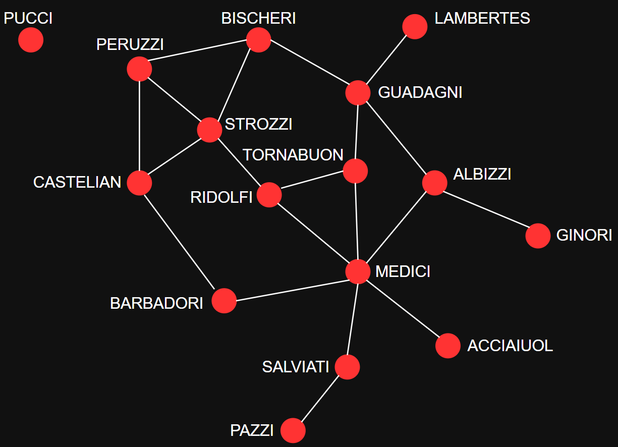
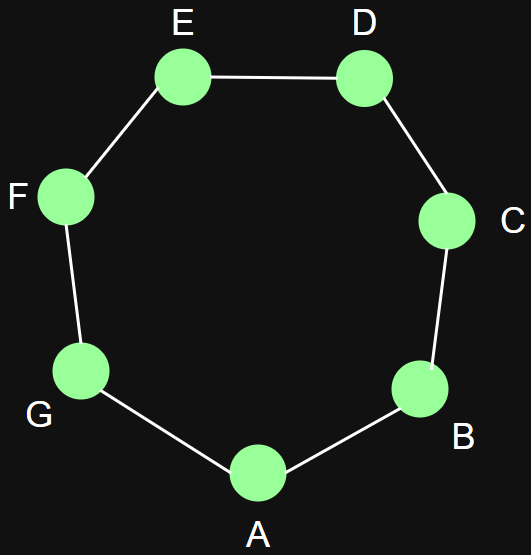
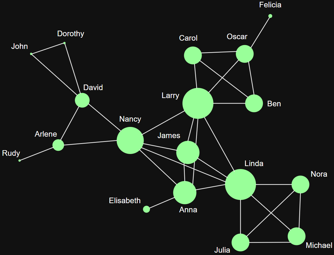
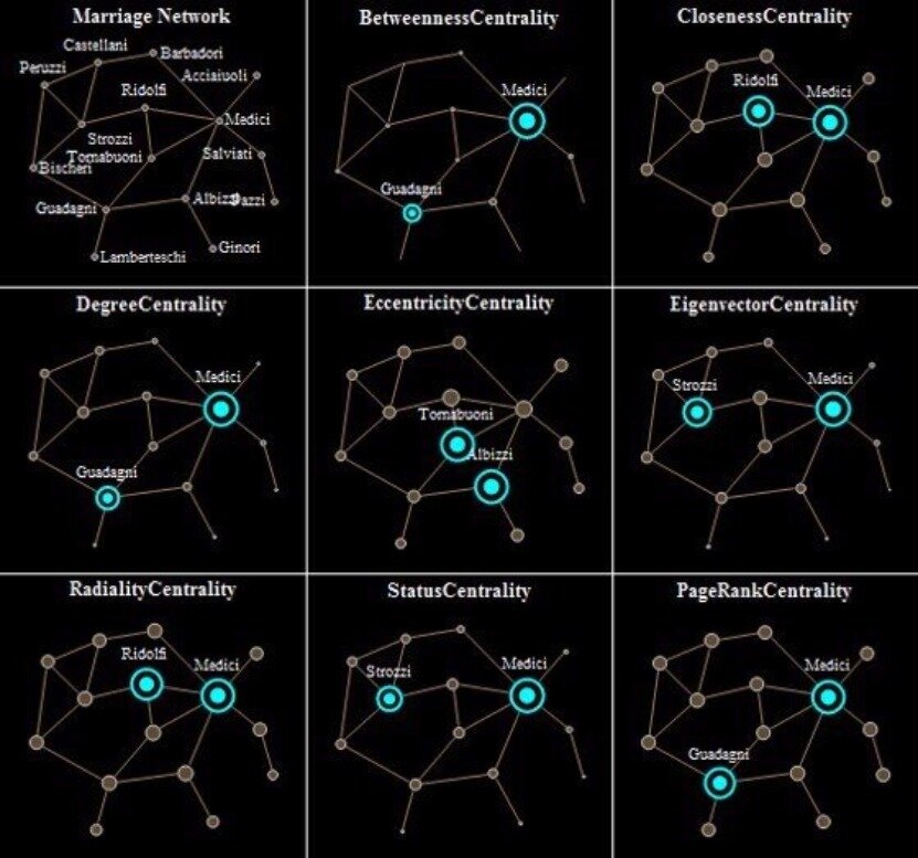
Marriage alliances among leading
Florentine families 15th century.
Determine the most ”important” or ”prominent” actors in the network based on actor location.
Some (obvious) examples
a)
b)
c)
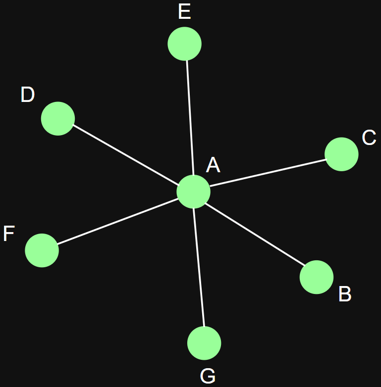

Degree centrality: number of nearest neighbors
Normalized degree centrality
High centrality degree -direct contact with many other actors
Degree Centrality
C_D(i)=k(i)=\sum_j A_{i j}=\sum_j A_{j i}
C_D^*(i)=\frac{1}{n-1} C_D(i)=\frac{k(i)}{n-1}
Closeness centrality: how close an actor to all the other actors in network
Normalized closeness centrality
High closeness centrality - short communication path to others, minimal number of steps to reach others
Closeness Centrality
C_C(i)=\frac{1}{\sum_j d(i, j)}
C_C^*(i)=(n-1) C_C(i)=\frac{n-1}{\sum_j d(i, j)}
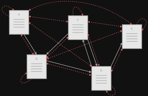
Betweenness centrality: number of shortest paths going through the actor σst(i)
Normalized betweenness centrality
Hight betweenness centrality - vertex lies on many shortest paths Probability that a communication from s to t will go through i
Betweenness Centrality
C_B(i)=\sum_{s \neq t \neq i} \frac{\sigma_{s t}(i)}{\sigma_{s t}}
C_B^*(i)=\frac{2}{(n-1)(n-2)} C_B(i)=\frac{2}{(n-1)(n-2)} \sum_{s \neq t \neq i} \frac{\sigma_{s t}(i)}{\sigma_{s t}}
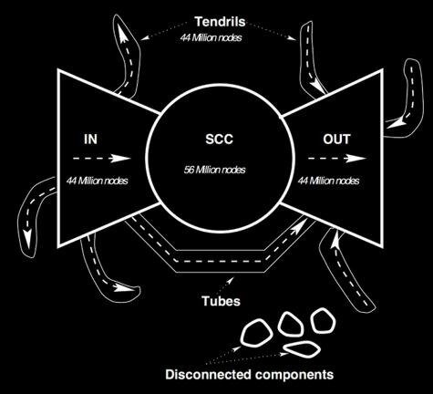
Bow-tie Structure
Importance of a node depends on the importance of its neighbors (recursive definition)
Select an eigenvector associated with largest eigenvalue λ = λ1, v = v1
Eigenvector Centrality
\begin{gathered}
v_i \leftarrow \sum_j A_{i j} v_j \\
v_i=\frac{1}{\lambda} \sum_j A_{i j} v_j \\
\mathbf{A} \mathbf{v}=\lambda \mathbf{v}
\end{gathered}
Closeness Centrality
Betweenness Centrality
Eigenvector Centrality
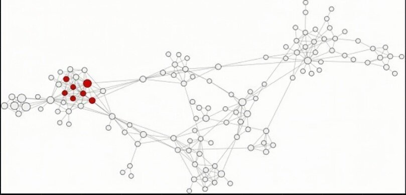
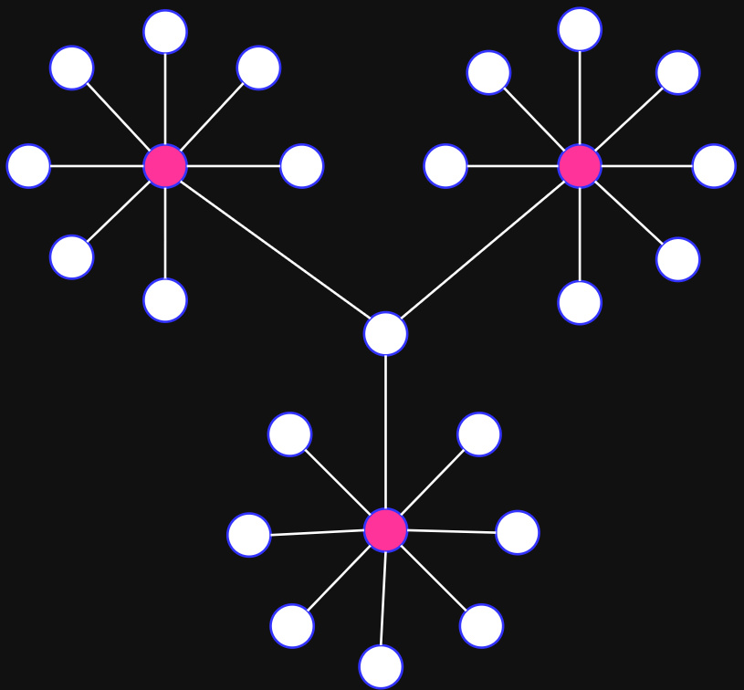
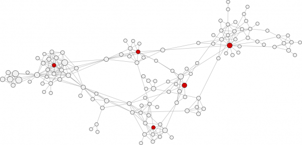
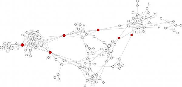
A) Degree centrality
B) Closeness centrality
D) Eigenvector centrality
C) Betweenness centrality
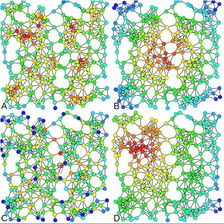
from Claudio Rocchini
Centrality Examples
Centralization (network measure) - how central the most central node in the network in relation to all other nodes.
\(C_x \) - one of the centrality measures
\(p_* \) - node with the largest centrality value
max - is taken over all graphs with the same number of nodes (for degree, closeness and betweenness the most centralizedstructure is the star graph)
Linton Freeman, 1979
Centralization
C_x=\frac{\sum_i^N\left[C_x\left(p_*\right)-C_x\left(p_i\right)\right]}{\max \sum_i^N\left[C_x\left(p_*\right)-C_x\left(p_i\right)\right]}
Directed graph: distinguish between choices made (outgoing edges) and choices received (incoming edges)
sending - receiving
export - import
cite papers - being cited
Directional Relations
Degree centrality (normalized):
Closeness centrality (normalised):
Betweenness centrality (normalized):
All based on outgoing edges
Centrality Measures
C_D^*(i)=\frac{k^{\text {out }}(i)}{n-1}
C_C^*(i)=\frac{n-1}{\sum_j d(i, j)}
C_B^*(i)=\frac{1}{(n-1)(n-2)} \sum_{s \neq t \neq i} \frac{\sigma_{s t}(i)}{\sigma_{s t}}
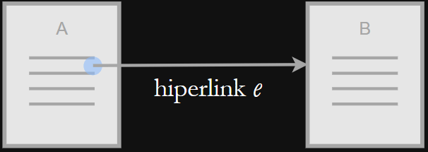
Hyperlinks - implicit endorsements
Web graph - graph of endorsements (sometimes reciprocal)
Web as a Graph
”PageRank can be thought of as a model of user behavior. We assume there is a ”random surfer” who is given a web page at random and keeps clicking on links, never hitting ”back” but eventually gets bored and starts on another random page. The probability that the random surfer visits a page is its PageRank.”
The anatomy of a large-scale hypertextual Web search engine Sergey Brin and Larry Page, 1998 [link]
Pagerank
Random Walk
Random walk on graph
With teleportation
Perron-Frobenius Theorem guarantees existence and uniqueness of the solution limt→∞ p = π
p_i^{t+1}=\sum_{j \in N(i)} \frac{p_j^t}{d_j^{\text {out }}}=\sum_j \frac{A_{j i}}{d_j^{\text {out }}} p_j
\begin{gathered}
\mathbf{P}=\mathbf{D}^{-1} \mathbf{A}, \quad \mathbf{D}_{i i}=\operatorname{diag}\left\{d_i^{\text {out }}\right\} \\
\mathbf{p}^{t+1}=\mathbf{P}^T \mathbf{p}^t
\end{gathered}
\mathbf{p}^{t+1}=\alpha \mathbf{P}^T \mathbf{p}^t+(1-\alpha) \frac{\mathbf{e}}{n}
\mathbf{p}=\alpha \mathbf{P}^T \mathbf{p}+(1-\alpha) \frac{\mathbf{e}}{n}
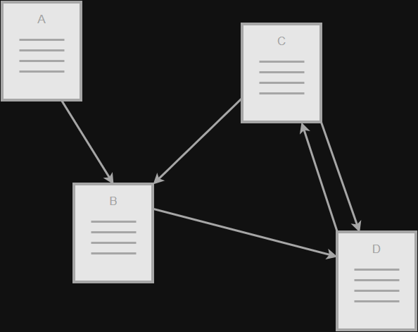
Pagerank
P R\left(p_i\right)=\frac{1-d}{N}+d \sum_{p_j \in M\left(p_i\right)} \frac{P R\left(p_j\right)}{L\left(p_j\right)}
\begin{array}{|c|c|c|c|c|}
\hline & \text { it 0 } & \text { it 1 } & \text { it 2 } & \text { PR } \\
\hline \text { A } & 1 / 4 & 1 / 12 & 1.5 / 12 & 1 \\
\hline \text { B } & 1 / 4 & 2.5 / 12 & 2 / 12 & 2 \\
\hline \text { C } & 1 / 4 & 4.5 / 12 & 4.5 / 12 & 4 \\
\hline \text { D } & 1 / 4 & 4 / 12 & 4 / 12 & 3 \\
\hline
\end{array}
\begin{array}{lll}
\text { 1. GeneRank } & \text { 13. TimedPageRank } & \text { 25. ImageRank } \\
\text { 2. ProteinRank } & \text { 14. SocialPageRank } & \text { 26. VisualRank } \\
\text { 3. FoodRank } & \text { 15. DiffusionRank } & \text { 27. QueryRank } \\
\text { 4. SportsRank } & \text { 16. ImpressionRank } & \text { 28. BookmarkRank } \\
\text { 5. HostRank } & \text { 17. TweetRank } & \text { 29. StoryRank } \\
\text { 6. TrustRank } & \text { 18. TwitterRank } & \text { 30. PerturbationRank } \\
\text { 7. BadRank } & \text { 19. ReversePageRank } & \text { 31. ChemicalRank } \\
\text { 8. ObjectRank } & \text { 20. PageTrust } & \text { 32. RoadRank } \\
\text { 9. ItemRank } & \text { 21. PopRank } & \text { 33. PaperRank } \\
\text { 10. ArticleRank } & \text { 22. CiteRank } & \text { 34. Etc... } \\
\text { 11. BookRank } & \text { 23. FactRank } & \\
\text { 12. FutureRank } & \text { 24. InvestorRank } &
\end{array}
Personalized PageRank (PPR) is a measure for node proximity on large graphs. For a pair of nodes s and t, the PPR value πs(t) equals the probability that an αdiscounted random walk from s terminates at t and reflects the importance between s and t in a bidirectional way
Personalized PageRank
Efficient Algorithms for Personalized PageRank Computation: A Survey, 2024, arxiv
\pi_{s} = (1 - \alpha) \mathbf{P} \pi_{s} + \alpha \cdot e_{s}
\pi_{s} = \alpha (\mathbf{I} - (1-\alpha)\mathbf{P})^{-1} e_{s}
is the indicator function. The degree matrix of \(G\) is an \(n \times n\) diagonal matrix \(mathbf{D}\) whose \(i\)-th diagonal entry equals \(d_{\text{out}}(v_i)\). The transition matrix of \(G\) is formalized as \(mathbf{P} = \mathbf{A}^\top \mathbf{D}^{-1}\). To ensure that \(mathbf{P}\) is well-defined, we assume that \(d_{\text{out}}(v) > 0\)
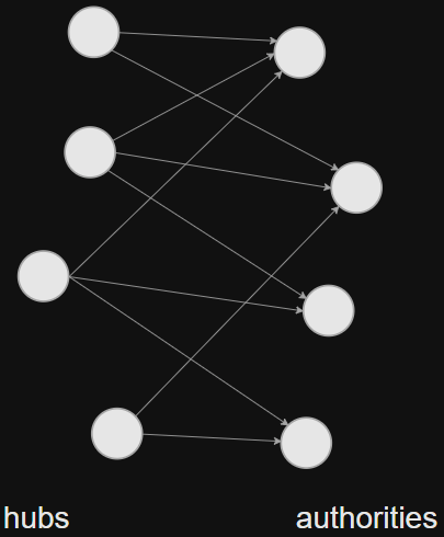
Hubs and Authorities (Hits)
Citation networks. Reviews vs original
research (authoritative) papers
authorities, contain uself information, ai
hubs, contains links to authorities, hi
Mutual recursion
good authorities referred bu good hubs
good hubs point to good authorities
a_i \leftarrow \sum_j A_{j i} h_j
h_i \leftarrow \sum_j A_{i j} a_j
Hubs and Authorities (Hits)
System of linear equation
Symmetric eigenvalue problem
where eigenvalue λ = (αβ)−1
\begin{aligned}
& \mathbf{a}=\alpha \mathbf{A}^T \mathbf{h} \\
& \mathbf{h}=\beta \mathbf{A} \mathbf{a}
\end{aligned}
\begin{aligned}
& \left(\mathbf{A}^T \mathbf{A}\right) \mathbf{a}=\lambda \mathbf{a} \\
& \left(\mathbf{A A}^T\right) \mathbf{h}=\lambda \mathbf{h}
\end{aligned}
Hubs and Authorities (Hits)
Hubs
Authorities
Centralities
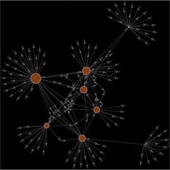
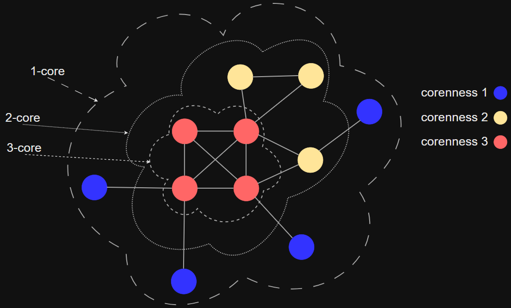
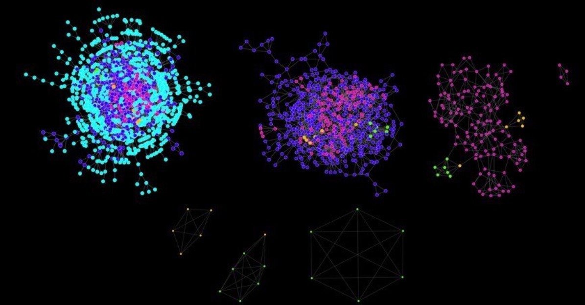
Core-Periphery Structure
image from J. Leskovec, K. Lang, 2010
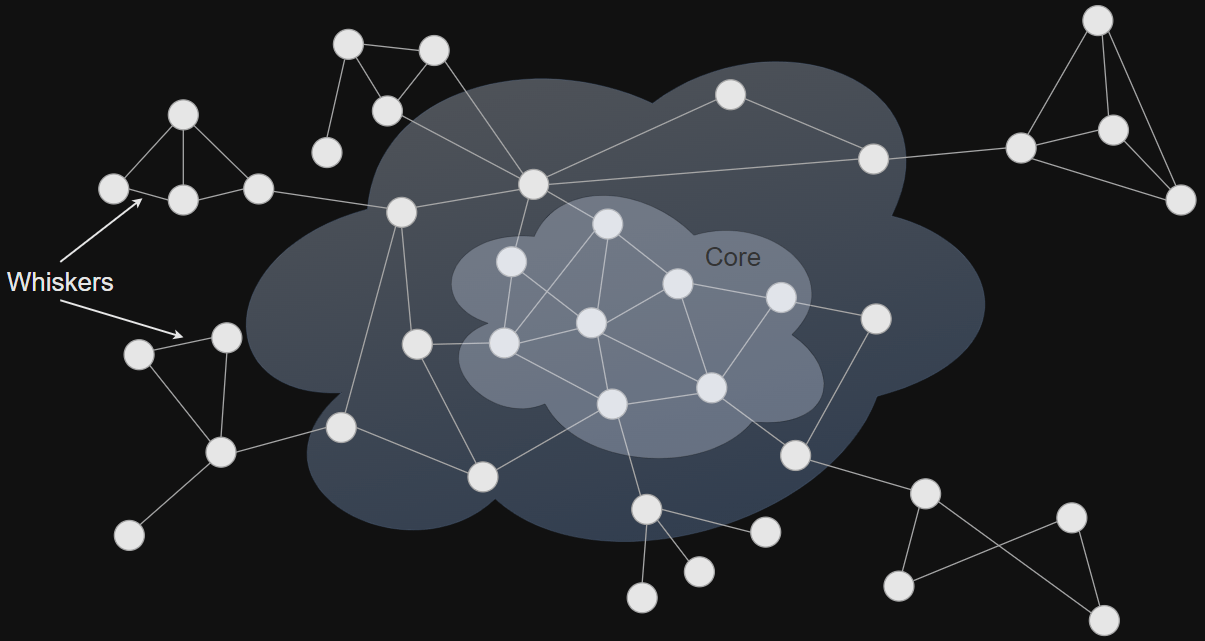
Graph Cores
A k-core is the largest subgraph such that each vertex is connected to at least k others in subset
Every vertex in k-core has a degree ki ≥ k
(k + 1)-core is always subgraph of k-core
The core number of a vertex is the highest order of a core that contains this vertex
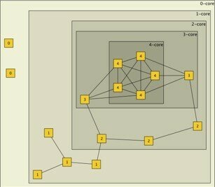
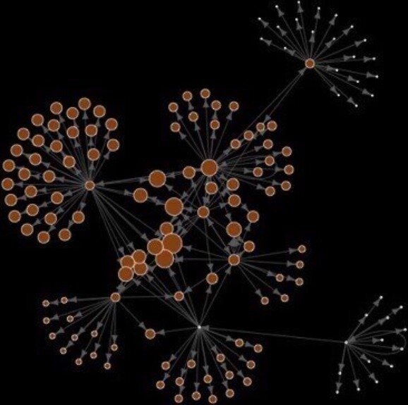
K-Cores
k-cores: 1:1458, 2:594, 3:142, 4:12, 5:6
k-shells: 1:864-red, 2:452-pale green, 3:130-green, 5:6-blue, 6:6-purple
R:graph.coreness(gcc)
K-Cores
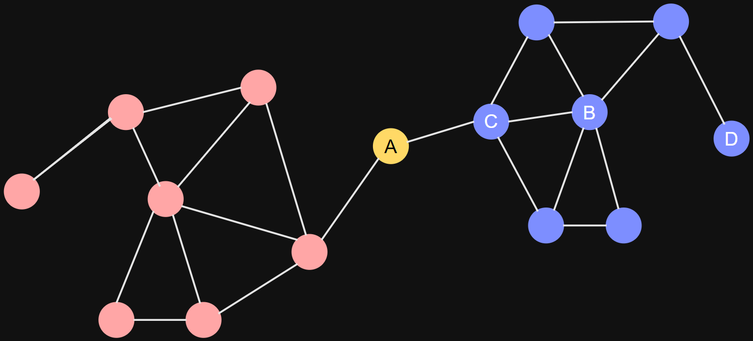
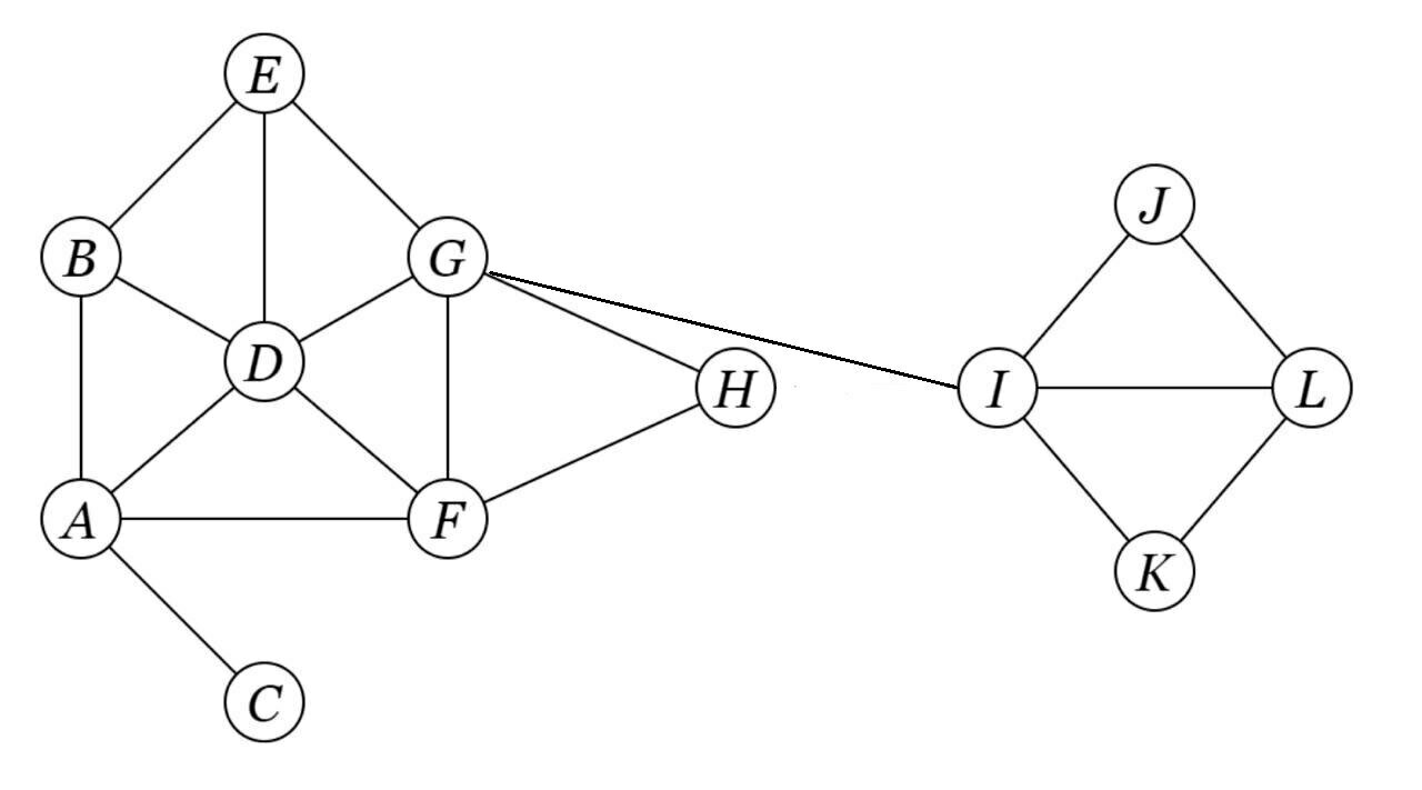
Find 3-core of the given network
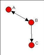
Dyads
Text
Dyad is a pair of vertices and possible relational ties between them:
- mutual
- asymmetric
- null (non-existent)
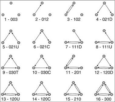
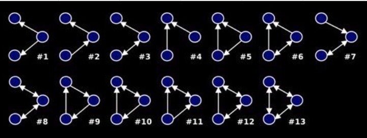
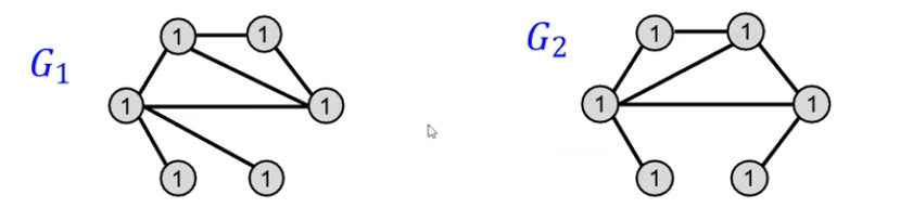
Triads
Triad is a subgraph of three vertices and possible ties between them:
Triad census :16 isomorphism classes
D - down, U - up, T - transitive, C - cyclic.
| mutual diads | assymetric dyads | null dyads |
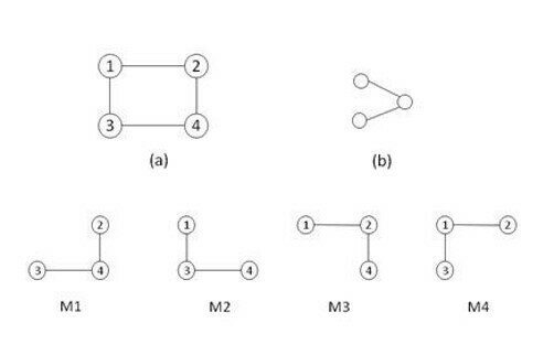
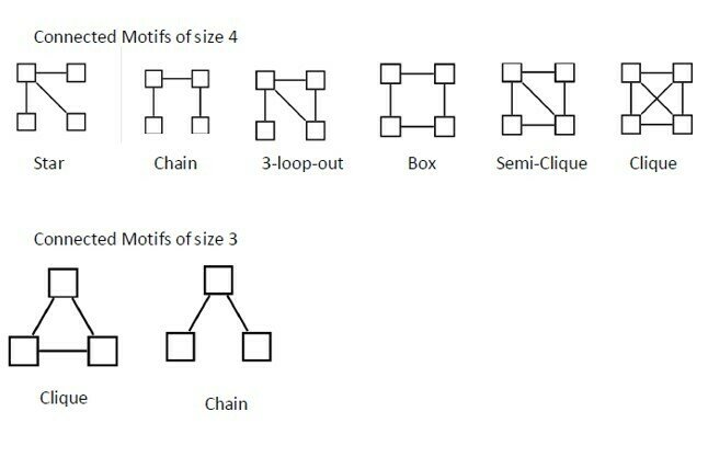
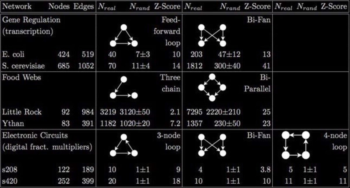
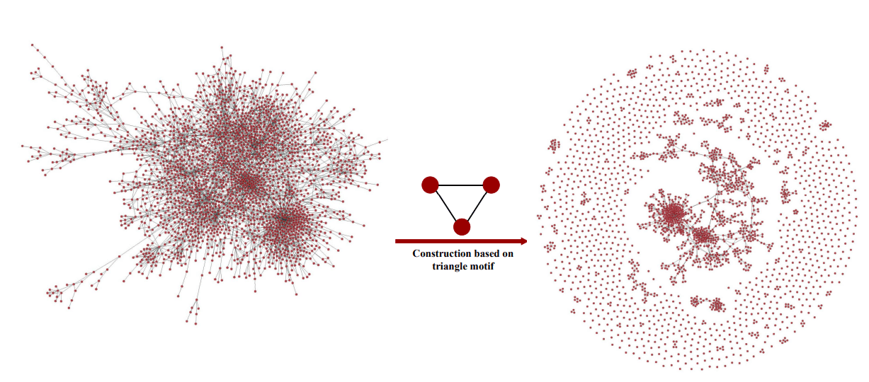
Network Motifs
Network motifs are recurrent statistically significant subgraphs or patterns in graphs connected subgraphs that (compare to random network)
Motifs are not induced subgraphs, i.e. they do not contain all the graph edges between selected vertices.
Network Motifs
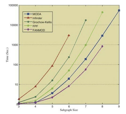
Motifs appear in a network more frequently than in a comparable random network
- calculate the number of occurrences of a sub graph
- evaluate the significance
For Gt subgraph (motif candidate) of G ,
R - random graph, µ - mean frequency, σ-standard deviatiom
Z_{\text {score }}\left(G^t\right)=\frac{F_G\left(G^t\right)-\mu_R\left(G^t\right)}{\sigma_R\left(G^t\right)}
Network Motifs
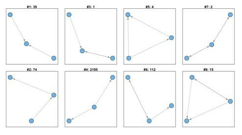
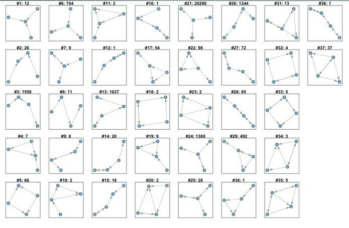
Undirected graphs: motifs of size 3 and 4
Network Motifs
Connected triads - motifs of size 3
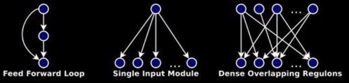
More complicated motifs:
Ribeiro, 2011, Shen-Orr, 2002
Network Motifs
S. Omidi, 2009
Network Motifs
Ribeiro, 2011, Milo, 2002
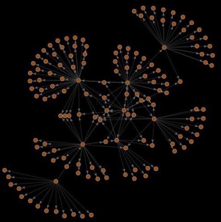
Network Motifs
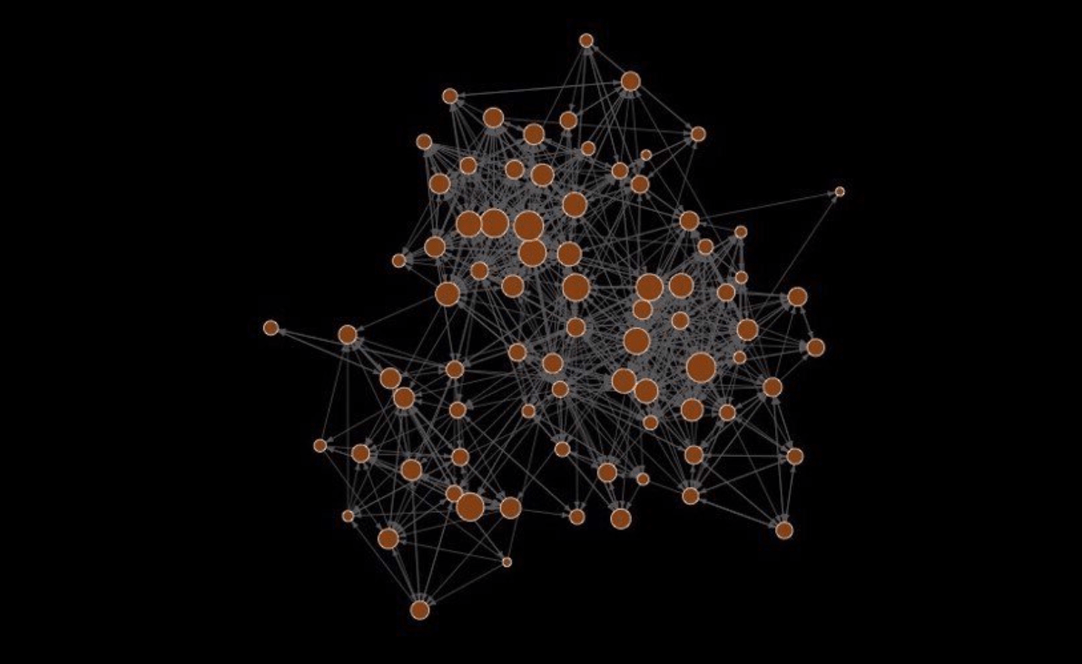
146 nodes, 187 edges
Network Motifs
Network Motifs
Network Motifs
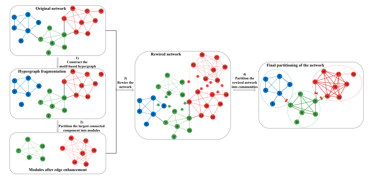
Network Motifs
References
- Centrality in Social Networks. Conceptual Clarification, Linton C. Freeman, Social Networks, 1, 215-239 , 1979
- Power and Centrality: A Family of Measures, Phillip Bonacich, The American Journal of Sociology, Vol. 92, No. 5, 1170-1182, 1987
- A new status index derived from sociometric analysis, L. Katz, Psychometrika, 19, 39-43, 1953.
- Eigenvector-like measures of centrality for asymmetric relations, Phillip Bonacich, Paulette Lloyd, Social Networks 23, 191-201 , 2001
- The PageRank Citation Ranking: Bringing Order to the Web. S. Brin, L. Page, R. Motwani, T. Winograd, Stanford Digital Library Technologies Project, 1998
- Authoritative Sources in a Hyperlinked Environment. Jon M. Kleinberg, Proc. 9th ACM-SIAM Symposium on Discrete Algorithms
- A Survey of Eigenvector Methods of Web Information Retrieval. Amy N. Langville and Carl D. Meyer, 2004
- PageRank beyond the Web. David F. Gleich, arXiv:1407.5107, 2014
Classical
Centralities
Graph Kernels
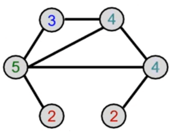
What if we use Bag of node degrees?
Deg1: Deg2: Deg3:
Both Graphlet Kernel and Weisfeiler-Lehman (WL) Kernel use Bag-of-* representation of graph, where * is more sophisticated than node degrees!
Graph Kernels
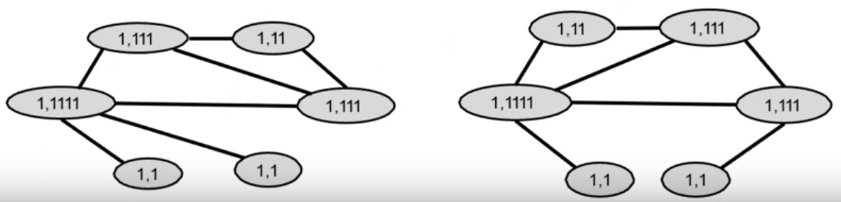
Given: A graph С with a set of nodes V.
- Assign an initial color с) (у) to each node v.
- Iteratively refine node colors by \(c^{(k+1)}(v)=HASH(\{ c^{(k)}(v),\{ c^{(k)}(u)\}_{u \in N(v)} \})\)
- where HASH maps different inputs to different colors.
- After К steps of color refinement, \(c^{(K)}(v)\) summarizes the structure of K-hop neighborhood
Graph Kernels
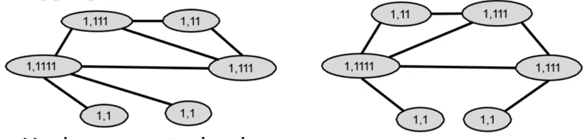
Given: A graph С with a set of nodes V.
- Assign an initial color с) (у) to each node v.
- Iteratively refine node colors by \(c^{(k+1)}(v)=HASH(\{ c^{(k)}(v),\{ c^{(k)}(u)\}_{u \in N(v)} \})\)
- where HASH maps different inputs to different colors.
- After К steps of color refinement, \(c^{(K)}(v)\) summarizes the structure of K-hop neighborhood
Graph Kernels
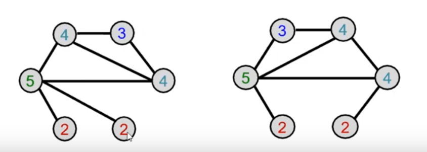
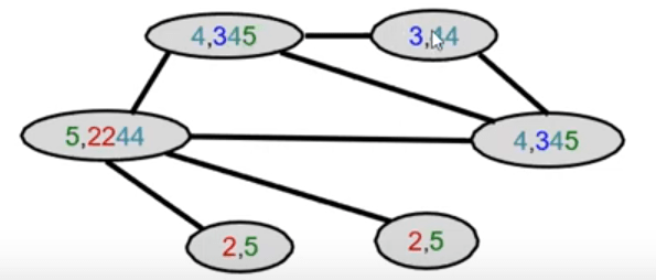
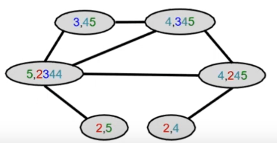
Aggregate neighboring colors
Assign initial colors
Graph Kernels
Hash aggregated colors
Aggregated colors
Graph Kernels
Hash aggregated colors
Aggregated colors
Graph Kernels
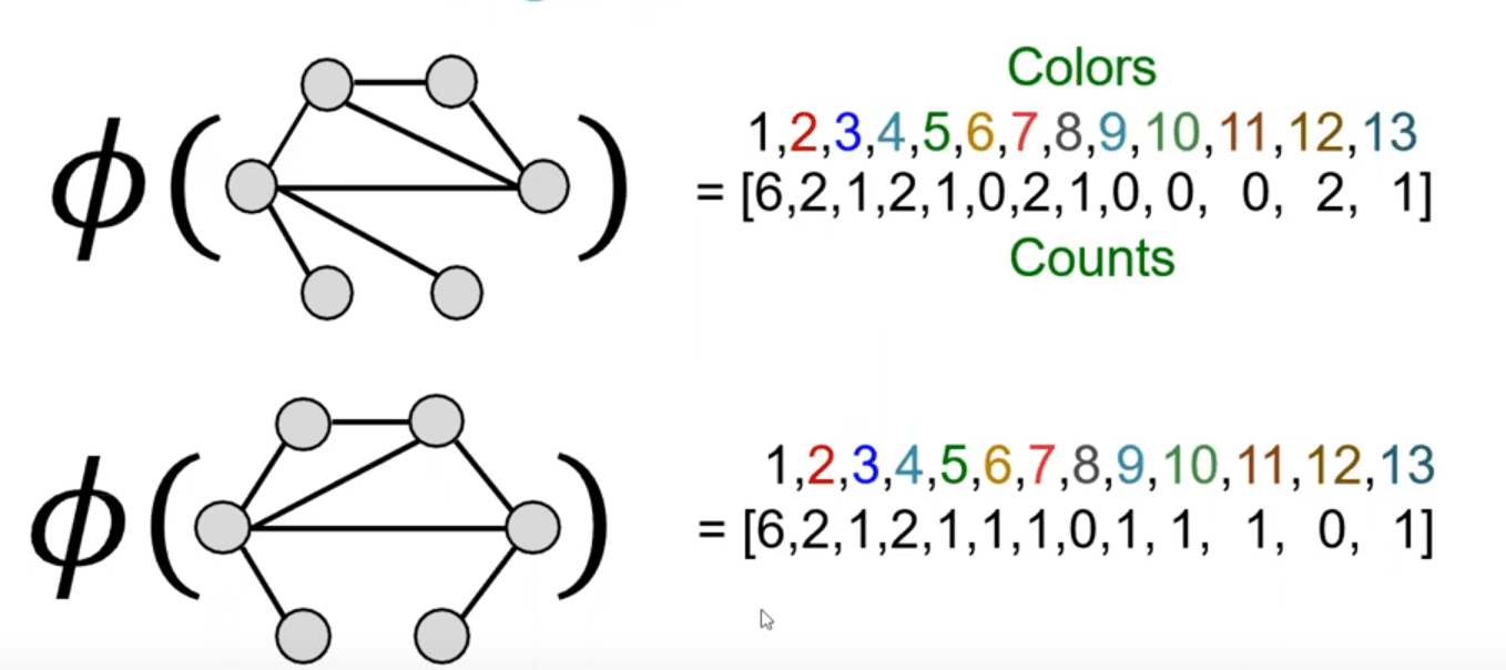
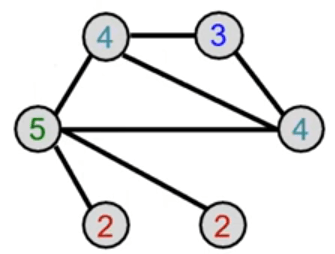
After color refinement, WL kernel counts number of nodes with a given color.
Degree centrality
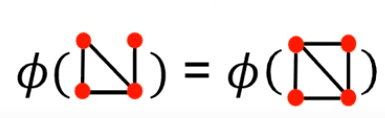
Key idea: Bag-of-Words (BoW) for a graph
- BoW simply uses the word counts as features for documents (no ordering considered).
- Naive extension to a graph: Regard nodes as words.
- Since both graphs have 4 red nodes, we get the same feature vector for two different graphs
2.01 Node Centralities
By karpovilia


