Recommendation systems
Week 8

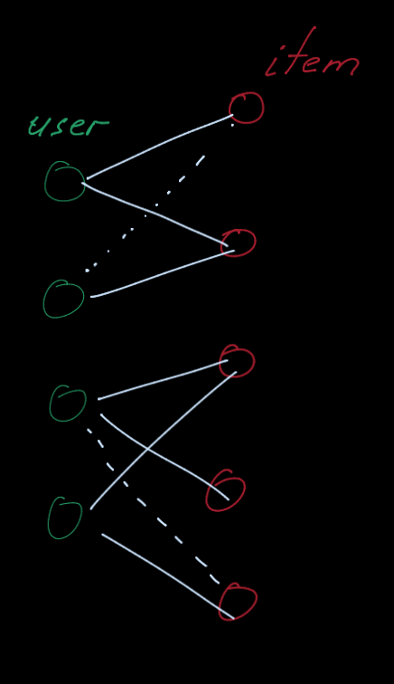
Recommender system can
modeled as a bipartite graph with two node types: users and items.
- Edges connect users and items and indicate user-item interaction
(e.g., click, purchase, review etc.)
- Often edge has timestamp of the interaction.

Given past user-item interactions we want to predict new items, the user will
interact in the future

- link prediction task

We need three functions:
- an encoder to generate user embeddings 𝒖
- an encoder to generate item embeddings 𝒗
- Score - a scalar function score(u, v), that returns a real-valued score

link prediction

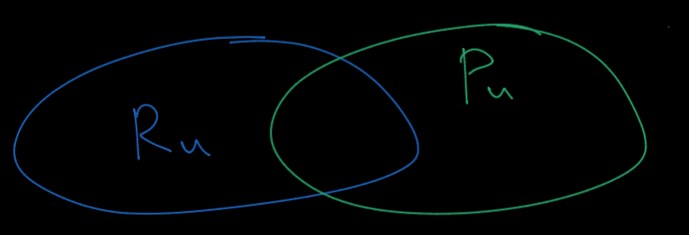
Evaluation metric

• \( P_u \) is a set of positive items the user will interace in the future.
• \( R_u \) is a set of items recommended by the model.
• In top-K recommendation, \( |R_u| = K \).
• Items that the user has already interacted are excluded.

Evaluation metric

The original training objective (recall@K) is not differentiable.

Two surrogate loss functions are widely-used to enable efficient gradient-based optimization.

• Binary loss
• Bayesian personalized Ranking (BPR) loss

Binary Loss

1. Define positive/negative edges

• A set of positive edges \( E \) (i.e., observed/training user-item interactions)
• A set of negative edges \( E_{neg} = {(u,v) | (u,v) \notin E, U \in U, v \in V} \)

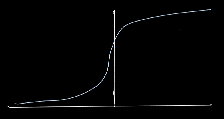
2. Define sigmoid function \( \sigma(x) = \frac{1}{1 + exp(-x)} \)

• Maps real-valued scores into binary likelihood  scores, i.e., in the range of [0,1].

Curriculum learning

• CuCo: Graph Representation with Curriculum Contrastive Learning
• On The Power of Curriculum Learning in Training Deep Networks
• Sampling Matters in Deep Embedding Learning
• FaceNet: A Unified Embedding for Face Recognition and Clustering

Binary Loss

Binary loss: Binary classification of positive/negative edges using \( 𝜎(𝑓, 𝒖, 𝒗 ) \):

\( -\frac{1}{|E|} \sum_{(u, v) \in E} \log \left(\sigma\left(f_\theta(\boldsymbol{u}, \boldsymbol{v})\right)\right)-\frac{1}{\left|E_{\mathrm{neg}}\right|} \sum_{(u, v) \in E_{\mathrm{neg}}} \log \left(1-\sigma\left(f_\theta(\boldsymbol{u}, \boldsymbol{v})\right)\right) \)

Binary loss pushes the scores of positive edges higher than those of negative edges.

• This aligns with the training recall metric since positive edges need to be recalled.Cae

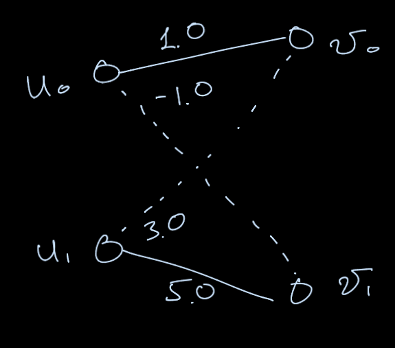
Binary Loss

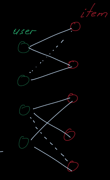
Let’s consider the simplest case: 

• Two users, two items 
• Metric: Recall@1. 
• A model assigns the score for every user-item pair (as shown in the right). 

Training Recall@1 is 1.0, because \( v_0 \)  is correctly recommended to \( u_0 \)

However, the binary loss would still penalize the model prediction because the negative \( (u_1, v_0) \) edge gets the higher score than \( (u_0, v_0) \)

  Bayesian Personalized Ranking

Positive edges for each user \( u^* \in U \)
\( \text { - } \boldsymbol{E}\left(u^*\right) \equiv\left\{\left(u^*, v\right) \mid\left(u^*, v\right) \in \boldsymbol{E}\right\} \)

Negative edges for each user  \( u^* \in U \)

\( \boldsymbol{E}_{\text {neg }}\left(u^*\right) \equiv\left\{\left(u^*, v\right) \mid\left(u^*, v\right) \in \boldsymbol{E}_{\text {neg }}\right\} \)

  Bayesian Personalized Ranking

For each user \( u^* \), we want the scores of rooted positive edges \( E(u^*) \) to be higher than those of rooted negative edges \( Е_{neg}(u^*) \).

  Bayesian Personalized Ranking

For each user \( u^* \), we want the scores of rooted positive edges \( E(u^*) \) to be higher than those of rooted negative edges \( Е_{neg}(u^*) \).

Final BPR Loss:  \( L = \frac{1}{|\boldsymbol{U}|} \sum_{u^* \in \boldsymbol{U}} \operatorname{Loss}\left(u^*\right) \)

Neural Graph Collaborative Filtering

Neural Graph Collaborative Filtering (NGCF) explicitly incorporates high-order graph structure when generating user/item embeddings.

Key idea: Use a GNN to generate graph-aware user/item embeddings

Initial shallow embeddings

(not graph-aware)

Use a GNN to propagate
embeddings

NGCF's graph-aware
embeddings

Neural Graph Collaborative Filtering

Forall \( u \in U \) , \( v \in V \), we set

 \( \boldsymbol{u} \leftarrow \boldsymbol{h}_u^{(K)}, \boldsymbol{v} \leftarrow \boldsymbol{h}_v^{(K)} \)

          Model             Venue       Year         Strategy

The most significant perfomance shift is in the order of 10e-3

GFCF is the best replicated model as it does not implement any random initialization of the weights

NGCF and DGCF ratele achieve 10e-4 because of the random initializations and stochastic learning processes involved