Social Network Analysis
week 02
Basic Concepts
Basic Concepts
Basic Concepts
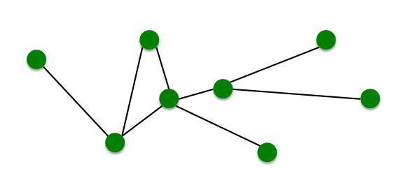
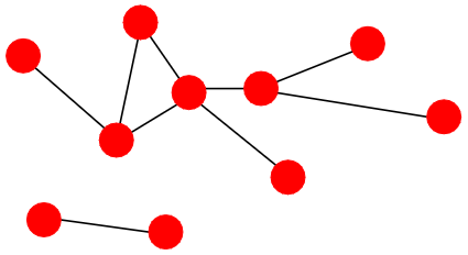
- A network is a collection of objects where some pairs of objects are connected by links
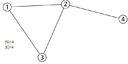
| Objects: nodes, vertices | N |
| Interactions: links, edges | E |
| System: network, graph | G(N,E) |
- A graph G = (V, E) is an ordered pair of sets: a set of vertices V and a set edges E, where n = |V|, m = |E|
- An edge eij = (vi, vj) is pair of vertices (ordered pair for directed graph)
Basic Concepts
- Network often refers to real systems like Web, Social network, Metabolic network
- Language: Network, node, link
- Graph is a mathematical representation of a network Web graph, Social graph (a Facebook term)
- Language: Graph, vertex, edge
How to define a network
How to build a graph:
- What are nodes?
- What are edges?
Choice of the proper network representation of a given domain/problem determines our ability to use networks successfully:
- In some cases there is a unique, unambiguous representation
- In other cases, the representation is by no means unique
- The way you assign links will determine the nature of the question you can study
How to define a network
Directed vs Undirected networks
Undirected Graphs
Links: undirected (symmetrical, reciprocal)
Examples: Collaborations Friendship on Facebook
Directed Graphs
Links: directed (arcs)
Examples: Phone calls Following on Twitter
The graph is called (un)directed iff. the set of pairs is (un)directed respectively.
Directed vs Undirected networks
The edge that consists of the same elements is called loop.
The subset of edges that consists of the same elements is called multiple edges (or multi-edge).
Two nodes/vertices are adjacent if they share a common edge An edge and a node on that edge are called incident.
Example:
(1, 1) — loop,
((1, 2),(1, 2),(1, 2)) — multiple edges.
Directed graph is called oriented graph if there are no two-side edges between any two vertices of the graph.
Graph Isomorphism
Two graphs are called isomorphic if one can re-number the vertices of one graph to obtain another.
Adjacency matrix
Two nodes/vertices are adjacent if they share a common edge An edge and a node on that edge are called incident.
Properties of adjacency matrix:
- Adjacency matrix is symmetrical for undirected graph
- Adjacency matrix diagonal elements equal to 0 (no loops)
- Adjacency matrix always square matrix
- For unweighted graph adjacency matrix consists of 0 and 1 and deg vi = {the sum of row i elements}
A(G)=\left\{a_{i j}\right\}:= \begin{cases}1 & \text { if there exists edge from vertex } v_i \text { to vertex } v_j \\ 0 & \text { otherwise }\end{cases}
Incidence matrix
Two nodes/vertices are adjacent if they share a common edge An edge and a node on that edge are called incident.
Properties of incidence matrix:
- In each column of incidence matrix there are only two non-zero elements
- Incidence matrix is rectangular matrix with dimensions ∥V ∥ × ∥E∥
- The sum of elements in each incidence matrix column equals to 0 for directed graphs
- For unweighted undirected graph incidence matrix consists of 0 and 1 and deg vi = {the sum of row i elements}
B(G)=\left\{b_{i j}\right\}=\left\{\begin{array}{ll}
1 & \text { if edge } j \text { starts from vertex } v_i \\
-1 & \text { if edge } j \text { ends in vertex } v_i \\
0 & \text { otherwise }
\end{array} .\right.
Incidence matrix
Two nodes/vertices are adjacent if they share a common edge An edge and a node on that edge are called incident.
For unweighted undirected graph incidence matrix is defined equivalently, but instead of -1 will be 1.
To generalize incidence matrix definition for weighted graphs (or weighted incidence matrix) multiply each column by weight of corresponding edge.
B(G)=\left\{b_{i j}\right\}=\left\{\begin{array}{ll}
1 & \text { if edge } j \text { starts from vertex } v_i \\
-1 & \text { if edge } j \text { ends in vertex } v_i \\
0 & \text { otherwise }
\end{array} .\right.
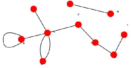
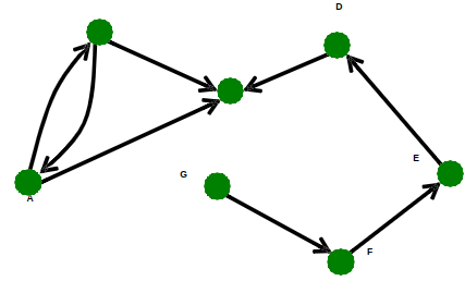
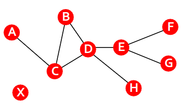
Graph Connectivity
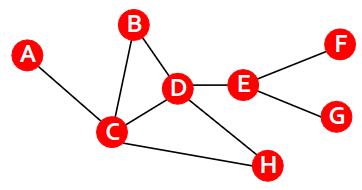
- Strongly connected directed graph has a path from each node to every other node and vice versa e.g., A-B path and B-A path)
- Weakly connected directed graph is connected if we disregard the edge directions
Graph on the left is connected but not strongly connected (e.g., there is no way to get from F to G by following the edge directions).
K-connectivity
A set of vertices (edges) is called k-vertex (edge) cut if a graph becomes not connected after the deletion of this set.
A graph is called κ-vertex (edge) connected iff. if it doesn’t have any k − 1-vertex (edge) cuts.
κ-vertex connectivity is also shortly called κ-connectivity.The paths between two vertices are called k-vertex (edge) independent iff. there exist k paths from it which consist of disjoint sets of vertices (edges).
Node Degree
Undirected Graphs
Node degree, : the number of edges adjacent to node i
Directed Graphs
Node degree = in-degree + out-degree.
k_i
\overline{k} = \langle k \rangle=\dfrac{1}{N}\sum_{i=1}^{N}{k_i}=\dfrac{2E}{N}
Complete Graph
The maximum number of edges in an undirected graph on N nodes is
E_{max}=\dfrac{N(N-1)}{2}
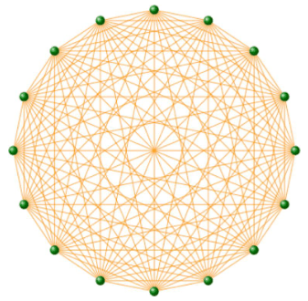
An undirected graph with the number of edges E = Emax is called a complete graph, and its average degree is N-1
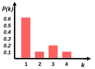
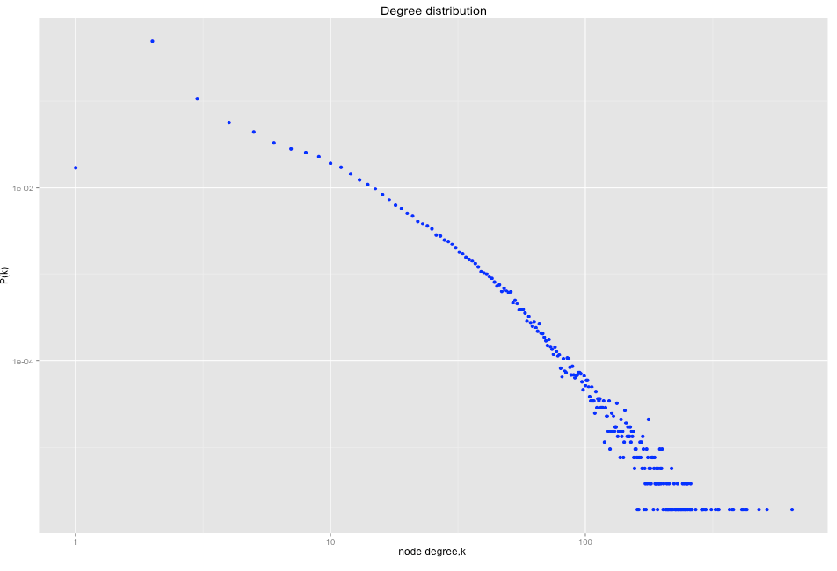
Degree distribution
Degree distribution \( P(k) \) :
Probability that a randomly chosen node has degree \( k \)
\( N_k \) - # nodes with degree \( k \)
P(k)=\dfrac{N_k}{N}
Power law distribution
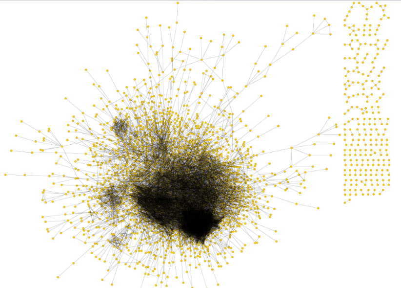
Power law distribution
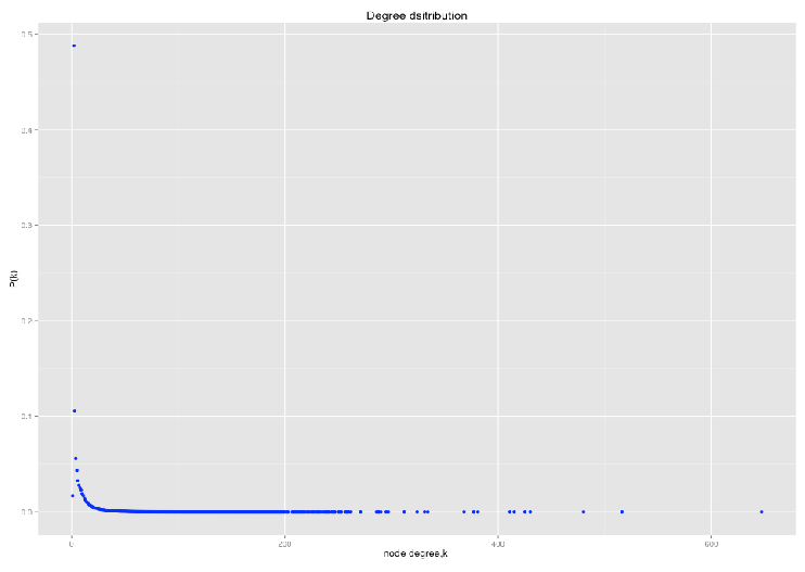
Power law distribution
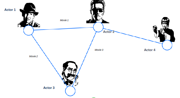
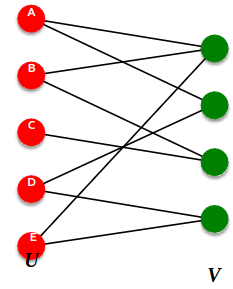
Bipartite Graph
Bipartite graph is a graph whose nodes can be divided into two disjoint sets U and V such that every link connects a node in U to one in V; that is, U and V are independent sets
Examples:
- Authors-to-Papers (they authored)
- Actors-to-Movies (they appeared in)
- Users-to-Movies (they rated)
- Recipes-to-Ingredients (they contain)
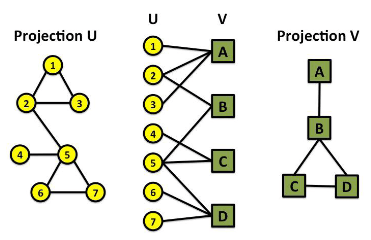
“Folded” networks:
- Author collaboration networks
- Movie co-rating networks
Bipartite Graph
Connected undirected graph is called bipartite iff. one can divide the vertices into two groups such that any two vertices from one group are not adjacent.
Consider the bipartite property testing algorithm:
- Choose any vertex.
- Start depth-first or breadth-first algorithms and divide vertices to 0 or 1 groups by putting to them corresponded marks:
- For depth-first: sequentially alternate marks for depth-first walk.
- For breadth-first: put the same marks if the vertices are on the same breadth and change marks otherwise.
- If any two vertices from one group are not adjacent, the graph is bipartite and not bipartite otherwise.
Bipartite Graph
Connected undirected graph is bipartite iff. it doesn’t contain odd length cycles.
1. Necessarity. Assume the contrary: the graph contains odd length cycle. Let’s start to divide vertices from this cycle to two groups by the rule: two vertices from one group should not be adjacent. By this rule vertices will sequentially alternate to each other. Since the length of cycle is odd, the first and the last vertices will be from the same group. This gives a contradiction with bipartite condition.
2. Sufficiency. Consider bipartite property testing algorithm with spanning tree T construction. It is easy to see that any tree is a bipartite graph. Let’s start to add remaining edges. Denote first edge by (v, w). Assume that vertices v and w corresponds to the same group by the testing algorithm. By the lemma 5 there exists unique path from v to w in T. Since the marks alternate to each other along this path by the algorithm, this path with the edge (v, w) form an odd length cycle. This gives a contradiction. Hence, all remaining edges connect vertices from different groups.
Bipartite Graph
Local and global characteristics of graph
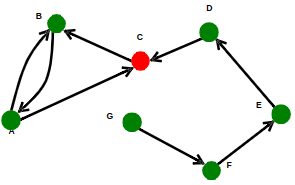
Path in Graphs
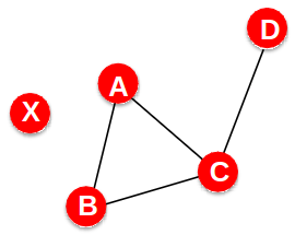
A path is a sequence of nodes in which each node is linked to the next one
P_n=\{i_0,i_1,i_2, ...,i_n\}
A path can intersect itself and pass through the same edge multiple times
E.g.: ACBDCDEG
P_n=\{(i_0,i_1)(i_1,i_2)(i_2,i_3), ..., (i_{n-1},i_n)\}
Path in Graphs
Cycle is a path consisted from distinct edges where the first and last vertices coincide.
Simple path is a path where any edges and vertices are distinct except the first and the last vertices.
Simple cycle is a simple path where the first and last vertices coincide.
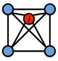
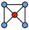
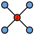
Node centrality
Centrality is a function defined for each vertex of a graph that contains some information of a graph structure.
Let’s denote by N(v) the set of vertices which adjacent to the vertex v. The simplest example is the degree centrality deg v = ∥N(v)∥.
Let’s denote by G(N(v)) the maximal sub-graph on vertices V (N(v)). Then MC(v) be the largest connected component in G(N(v)). Maximum neighborhood component MNC(v) is the number of vertices in MC(v).
Density of maximum neighborhood component DMNC(v) = ∥E(MC(v))∥ ∥V (MC(v))∥ ϵ , for some ϵ ∈ [1, 2].
Global characteristics of a graph
5. Average clustering coefficient:
C(G)=\frac{1}{\|V(G)\|} \sum_{v \in V(G)} C(v)=\frac{1}{\|V(G)\|} \sum_{v \in V(G)} \frac{2\|E(N(v))\|}{\operatorname{deg}(v)(\operatorname{deg}(v)-1)}
2. Density:
D(G)=\frac{\text { number of edges in } G}{\text { maximum possible number of edges in } G}=\frac{2 \| E(G)) \|}{\|V(G)\|(\|V(G)\|-1)}
1. The simplest example is the diametre:
3. Global efficiency:
4. Average shortest path length:
E_{g l o b}(G)=\frac{1}{\|V(G)\|(\|V(G)\|-1)} \sum_{s \neq t} \frac{1}{\operatorname{dist}(s, t)}
L(G)=\frac{1}{\|V(G)\|(\|V(G)\|-1)} \sum_{s \neq t} \operatorname{dist}(s, t)
diam(G) = max_{s,t} dist(s, t)
6. Small world coefficient:
SW(G) = \frac{C(G)}{C(G_{rand})} / \frac{L(G)}{L(G_{rand})}
where \(G_{rand}\) is a random graph \((|V(G)|, |E(G)|)\)
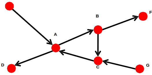
Distance in Graphs
Distance (shortest path, geodesic) between a pair of nodes is defined as the number of edges along the shortest path connecting the nodes
In directed graphs, paths need to follow the direction of the arrows Consequence: Distance is not symmetric:
If the two nodes are not connected, the distance is usually defined as infinite (or zero)
h_{B,C}\neq h_{C,B}
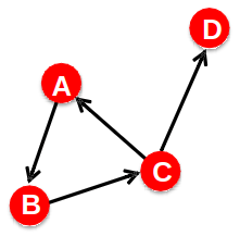
h_{B,D}=2
h_{B,C} = 1
h_{C,B} = 2
h_{A,X}=\infty
Network Diameter
- The distance between two vertices is the number of edges in the shortest path from vi to vj
- Graph diameter is the largest shortest path:
- Average path length:
\langle L \rangle=\dfrac{1}{n(n-1)}\sum_{i \neq j}{d_g(V_i,V_j)}
d_{G(v_i,vj)}
D = \max_{i,j}{d_{G(v_i,v_j)}}
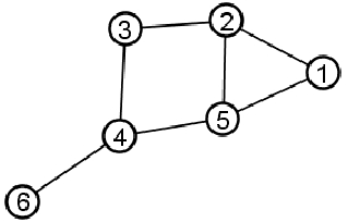
Global CC (Transitivity)
Global clustering coefficient:
C_Δ = \dfrac{3 \times {number \: of \: triangles}}{number \: of \: connected \: triplets \: of \: vertices}
\langle C \rangle = \dfrac{13}{42}\approx 0.310
C_Δ = \dfrac{3}{8}\approx 0.375
Local CC
Local clustering coefficient (per vertex)
How connected are i’s neighbors to each other?
C_i = \dfrac{2 e_i}{k_i(k_i-1)}
C_i = 1
C_i = \dfrac{1}{2}
C_i = 0
where ei is the number of edges between the neighbors of node i
Average CC
Average clustering coefficient
How connected are i’s neighbors to each other?
k_B = 2
\overline{C} = \dfrac{1}{N}\sum_{i=1}^{N}{C_i}
e_B = 1
C_B = 2/2 = 1
k_D = 4
e_D = 2
C_D = 4/12 = 1/3
Graph Laplacian
Laplacian Operator
L_{ij} =
\begin{cases}
d_i & \text{ if } i=j\\
-1 & \text{if $(i,j) \in \large\varepsilon = \delta_{ij} d_i - A_{ij} $ }\\
0 & \text{otherwise}
\end{cases}
L = D - A
D = \begin{bmatrix}
d_1 & 0 & \dots & 0 \\
0 & d_2 & & 0 \\
\vdots & & \ddots & 0 \\
0 & 0 & \dots & d_N
\end{bmatrix}
Laplacian Operator
L_{ij} =
\begin{cases}
d_i & \text{ if } i=j\\
-1 & \text{if $(i,j) \in \large\varepsilon = \delta_{ij} d_i - A_{ij} $ }\\
0 & \text{otherwise}
\end{cases}
L = D - A
Laplacian Operator
- Laplacian operator in physics is an "average difference between a point and a small sphere around that point"
- In a discrete case (the graph case), it is the difference between a node's value and its neighbors values
M. Bronstein, Geometric deep learning: going beyond Euclidean data, 2017
(Lx)_i = \sum_j(\delta_{ij}d_i - A_{ij})x_j
= d_i x_i - \sum_j{A_{ij}x_j}
= \sum_j{A_{ij}(x_i-x_j)}
= \sum_{(i,j)\in \epsilon}(x_i - x_j)
Properties of the Laplacian
- Every row sums to 0:
(L1)_i = \sum_jL_{ij}
= d_i - \sum_j{A_{ij}}
- I.e. 1 is an eigen-vector of L with eigen-value = 0
= \sum_j(\delta_{ij}d_i - A_{ij})
= d_i - d_i = 0
L1 = 0 = \lambda 1
where
\lambda = 0
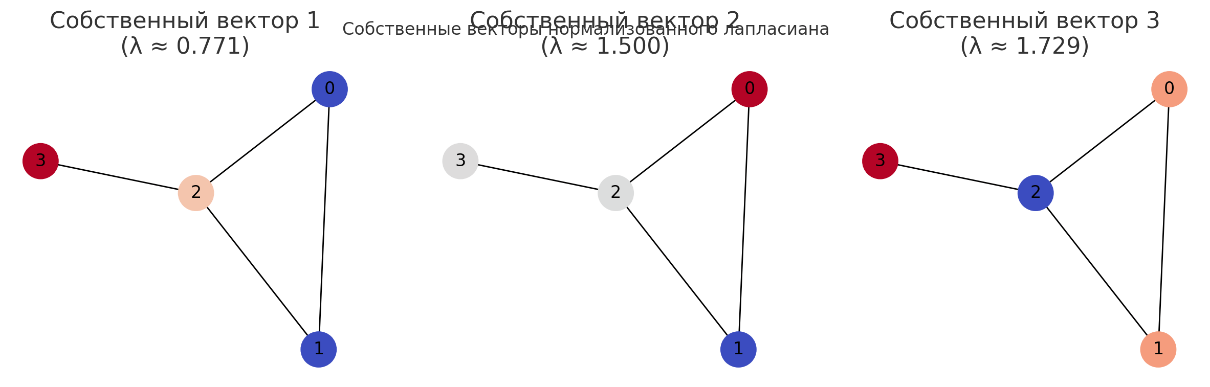
Normalized Laplacian
The normalized Laplacian matrix \(\Delta\) is defined as \(D^{-\frac{1}{2}}LD^{-\frac{1}{2}}\), where \(L\) is the Laplacian matrix of \(G\), and \(D = diag(deg \ v_1, \dots, deg \ v_n)\) is the diagonal matrix consisting of degrees of \(G\). Then the \((i, j)\)-entry of \(\Delta\) is
\begin{cases}1, & \text { if } i=j \\ -\frac{1}{\sqrt{d_i d_j}}, & \text { if } i \neq j,\{i, j\} \in E(G) \\ 0, & \text { otherwise }\end{cases}
in which we simply write \(d_i = deg \ v_i\) for convenience.
Properties of normalized Laplacian matrix
1. By viewing \(\Delta\) as a linear operator \(\Delta : \mathbb{R}^n \to \mathbb{R}^n\), \(\Delta\) is self-adjoint with respect to the scalar product \((\cdot, \cdot)\), i.e.,
\((x,\Delta y)\) = \((\Delta x, y)\)
for all \(x, y \in \mathbb{R}^n\). Here the scalar product is defined for pairs of vectors; formally, for any \(x, y \in \mathbb{R}^n\), \((x, y) := \sum_{i=1}^{n} x_i y_i\).
2. \(\Delta\) is non-negative:
\((\Delta x, x) \ge 0\), for all \(x\).
3. \(\Delta x = 0\) precisely when \(x\) is a vector collinear to \((\sqrt{d_1}, \dots, \sqrt{d_n})\).
4. The trace of \(\Delta\) is \(n\).
Normalized Laplacian
The normalized Laplacian matrix \(\Delta\) is defined as \(D^{-\frac{1}{2}}LD^{-\frac{1}{2}}\), where \(L\) is the Laplacian matrix of \(G\), and \(D = diag(deg \ v_1, \dots, deg \ v_n)\) is the diagonal matrix consisting of degrees of \(G\). Then the \((i, j)\)-entry of \(\Delta\) is
Graph Partitioning

Graph Partitioning
L \begin{bmatrix}
1 \\
1 \\
\vdots \\
0 \\
0 \\
\end{bmatrix}
= \lambda_1
\begin{bmatrix}
1 \\
1 \\
\vdots \\
0 \\
0 \\
\end{bmatrix}
\text{ where } \lambda_1 = 0
L \begin{bmatrix}
0 \\
0 \\
\vdots \\
1 \\
1 \\
\end{bmatrix}
= \lambda_2
\begin{bmatrix}
0 \\
0 \\
\vdots \\
1 \\
1 \\
\end{bmatrix}
\text{ where } \lambda_2 = 0
Graph Partitioning
e_0 = - \dfrac{1}{\sqrt{7}}
\begin{bmatrix}
1 \\
1 \\
0 \\
1 \\
1 \\
1 \\
1 \\
0 \\
0 \\
0 \\
0 \\
1 \\
\end{bmatrix}
e_1 = - \dfrac{1}{\sqrt{7}}
\begin{bmatrix}
0 \\
0 \\
1 \\
0 \\
0 \\
0 \\
0 \\
1 \\
1 \\
1 \\
1 \\
0 \\
\end{bmatrix}
\lambda_0 = \lambda_1 = 0
Positive semi-definite
x^TLx = \sum_{ij} L_{ij} x_i x_j
= \sum_{ij}(\delta_{ij}-A_{ij}) x_i x_j
= \dfrac{1}{2} \sum_i{d_i x_i^2} + \dfrac{1}{2} \sum_i{d_j x_j^2} -\sum_{ij}{A_{ij} x_i x_j}
= \dfrac{1}{2} \sum_{ij}{[A_{ij}x_i^2 - 2A_{ij}x_ix_j + A_{ij}x_j^2]}
x^TLx= \dfrac{1}{2} \sum_{ij}{A_{ij}(x_i - x_j)^2} \geq 0
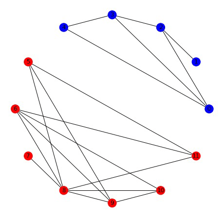
Node clustering
- Let x be a vector that is +1 if part of cluster A and -1 if part of cluster B
- Is 0 if \( x_i \) and \( x_j \) are in same cluster and 2 if they're in different clusters
If we find the \( x \) that minimizes this, we will find cluster assignments that minimize cross-cluster edges
x^TLx = \dfrac{1}{2} \sum_{ij}A_{ij}(x_i-x_j)^2 \geq 0
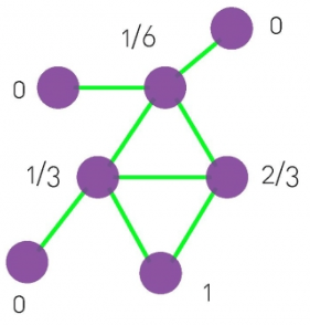
Node clustering
- If x is real-valued rather than +/- 1, we can more easily optimize and get a 1-dimensional embedding of nodes where we are minimizing the distance between connected nodes
- Need additional constraints because constant vector (c, c, …, c) is eigen-vector with eigen-value = 0, but that is trivial solution
x^TLx = \dfrac{1}{2} \sum_{ij}A_{ij}(x_i-x_j)^2 \geq 0
Node clustering
- Additional Constraints:
- Center of Mass about the origin:
- x.T*x = 1 so all points are not mapped to 0
- Rayleigh-Ritz theorem says solution is equal to eigen-vector with
- smallest eigen-value. (Makes intuitive sense)
- Smallest doesn’t fit our constraints
- Second smallest does (orthogonal to 1 and normalized)
- “Fiedler Vector”
x^TLx = \dfrac{1}{2} \sum_{ij}A_{ij}(x_i-x_j)^2 \geq 0
\sum_i x_i = 0 = x\bold{1} \leftrightarrow x \perp 1
Node clustering
- Turn into cluster assignment by taking sign of value in Fiedler vector
x =
\begin{bmatrix}
-0.5 \\
0.2 \\
-0.1 \\
0.3 \\
\end{bmatrix}
\rightarrow
\begin{bmatrix}
-1 \\
1 \\
-1 \\
1 \\
\end{bmatrix}
= \hat{x}
Node clustering
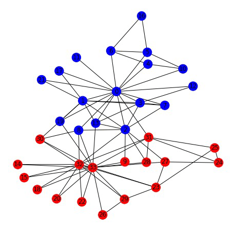
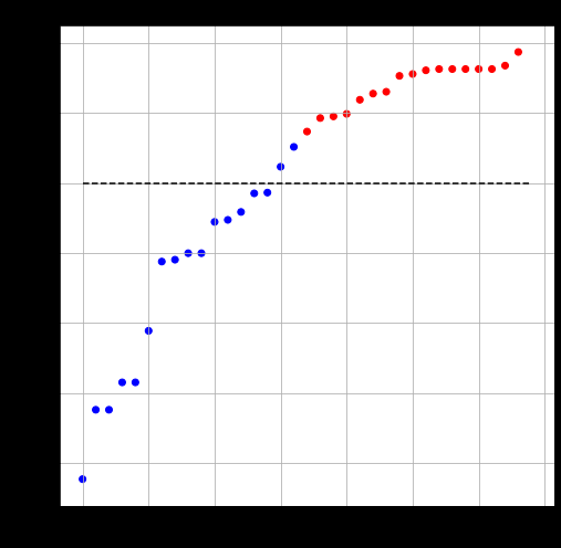
Karate club network
Fiedler Vector
Laplacian Operator Example
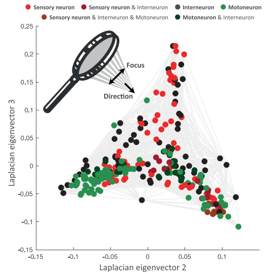
Javer, An open-source platform for analyzing and sharing worm-behavior data, Nature, 2018
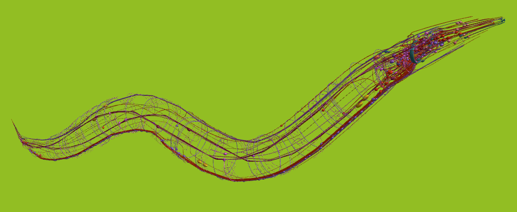
OpenWorm project
OpenWorm project visualization
The first comprehensive computational model of Caenorhabditis elegans (C. elegans), a microscopic roundworm. With only a thousand cells, it solves basic problems such as feeding, mate-finding and predator avoidance.
References
- Bondy, J. A. (2008). USR Murty Graph Theory. Graduate Texts in Mathematics, 244. [pdf]
- XU, Y. (2017). KURATOWSKI’S THEOREM. [pdf]
- Patrignani, M. (2013). Planarity Testing and Embedding. [pdf]
- Tutte, W. T. (1956). A theorem on planar graphs. Transactions of the American Mathematical Society, 82(1), 99-116. [pdf]
- Thomassen, C. (1983). A theorem on paths in planar graphs. Journal of Graph Theory, 7(2), 169-176. [pdf]
- KENDALL, M. STEINITZ’THEOREM FOR POLYHEDRA. [pdf]
- Strang, A., Haynes, O., Cahill, N. D., Narayan, D. A. (2018). Generalized relationships between characteristic path length, efficiency, clustering coefficients, and density. Social Network Analysis and Mining, 8, 1-6. [pdf]
- Chin, C. H., Chen, S. H., Wu, H. H., Ho, C. W., Ko, M. T., Lin, C. Y. (2014). cytoHubba: identifying hub objects and sub-networks from complex interactome. BMC systems biology, 8(4), 1-7. [pdf]
- Cvetkovi´c, D., Rowlinson, P., Simi´c, S. (2009). An Introduction to the Theory of Graph Spectra (London Mathematical Society Student Texts). Cambridge: Cambridge University Press [pdf]
- S. Amghibech, Eigenvalues of the discrete p-Laplacian for graphs. Ars Comb. 67 (2003), 283-302. [pdf]
Basic Concepts
By karpovilia


