Mathematical analysis of
data assimilation
Kota Takeda
(Kyoto University / RIKEN)
& related topics
Kota Takeda
PhD Student at Kyoto University

Junior Research Associate at RIKEN
Mathematics
Data Assimilation
Position

Kota Takeda 2
Activities
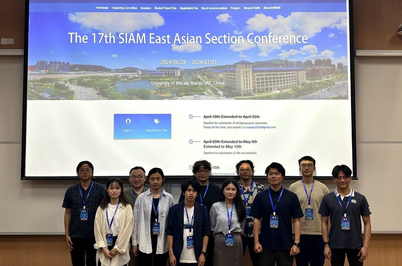
Organized MS at EASIAM 2024 Macao!

Advisor for high-school students
Volunteer at NPO clack
Cooperation with Leave a Nest Co., Ltd.
Teach programming
Assist students' research activities

See my website
Marathon

Finished Kobe marathon!
- Self-introduction ✓
- Data Assimilation/My research
- Related topics
This talk
Data Assimilation (DA)
The seamless integration of data and models
Model
Dynamical systems and its numerical simulations
ODE, PDE, SDE,
Numerical analysis, HPC,
Fluid mechanics, Physics
chaos
error
Data
Obtained from experiments or measurements
Statistics, Data analysis,
Radiosonde/Radar/Satellite observation
noise
limited
×


Each has Uncertainty! (incomplete)
Data Assimilation (DA)
-
Control
- Nudging/Continuous Data Assimilation
-
Bayesian
- Particle Filter (PF)
- Ensemble Kalman filter (EnKF)
-
Variational
- Four-dimensional Variation method (4DVar)
Several formulations & algorithms of DA:
current study
→ next slide
Numerical Weather Prediction
typical application


×
Setup: Model
Model dynamics in
Semi-group in

generates
(assume)
: separable Hilbert space
: separable Hilbert space (state space)
The known model generates
the unknown true chaotic orbit.


A small perturbation can
grow exponentially fast.
unknown orbit
Setup: Observation
Discrete-time model (at obs. time)

We have noisy observations in
Noisy observation
observe
...
bounded linear
(another Hilbert space).
Aim of Data Assimilation
Unkown state
Given obs.
Construct
estimate
Quality Assessment
Given
Model
Obs.
Obs.
unknown
(filtering problem)
Bayesian Data Assimilation
(I) Prediction
by Bayes' rule
by model
(II) Analysis
We can compute it iteratively (2 steps at each time step).
Prediction
...


(I) Prediction
(II)Analysis

Goal: compute the conditional distribution
Need approximations!
Repeat (I) & (II)
→ next slide
- Two major implementations of EnKF:
- Perturbed Observation (PO): stochastic → sampling error
- Ensemble Transform Kalman Filter (ETKF): deterministic
Ensemble filters

...
Repeat (I) & (II)
(II)Analysis
(I) Prediction


Particle Filter(PF)
→ full distribution
Ensemble Kalman filter (EnKF)
→ mean & Covariance
(Burgers+1998)
(Bishop+2001)
A set of state vectors
Mathematical analysis of EnKF
Assumptions on model
(Reasonable)
Assumption on observation
(Strong)
We focus on finite-dimensional state spaces
(T.+2024) K. T. & T. Sakajo (accepted 2024), SIAM/ASA Journal on Uncertainty Quantification.
Assumptions for analysis
Assumption (obs-1)
"full observation"
Strong!
Assumption (model-1)
Assumption (model-2)
Assumption (model-2')
Reasonable
"one-sided Lipschitz"
"Lipschitz"
"bounded"
or
Dissipative dynamical systems
Dissipative dynamical systems
Lorenz 63, 96 equations, widely used in geophysics,
Example (Lorenz 96)
non-linear conserving
linear dissipating
forcing
Assumptions (model-1, 2, 2')
hold
incompressible 2D Navier-Stokes equations (2D-NSE) in infinite-dim. setting
Lorenz 63 eq. can be written in the same form.
→ We can discuss ODE and PDE in a unified framework.
can be generalized
bilinear operator
linear operator
dissipative dynamical systems
Mimics chaotic variation of
physical quantities at equal latitudes.
(Lorenz1996) (Lorenz+1998)
Dissipative dynamical systems
The orbits of the Lorenz 63 equation.
Literature review: analysis of EnKF
Error analysis for dissipative dynamical systems
-
Full observation ( )
-
PO + add. inflation (Kelly+2014)
-
ETKF + multi. inflation (T.+2024)
-
-
Partial observation → future
asmp obs1
asmp model1
asmp model2
asmp model2'
How EnKF approximate
the true state?
→ current
-
Consistency (Mandel+2011, Kwiatkowski+2015)
-
Sampling errors (Al-Ghattas+2024)
How EnKF approximate KF?
Analysis for linear-Gaussian systems
Error analysis of ETKF (our)
(T.+2024) K. T. & T. Sakajo (accepted 2024), SIAM/ASA Journal on Uncertainty Quantification.
Theorem 2 (T.+2024)
Sketch: Error analysis of ETKF

①
②
Key result
Data Assimilation (DA)
-
Control
- Nudging/Continuous Data Assimilation
-
Bayesian
- Particle Filter (PF)
- Ensemble Kalman filter (EnKF)
- Quantum DA
-
Variational
- Four-dimensional Variation method (4DVar)
PDE
Optimal Transport
Metrics
Machine
Learning
Diffusion model
Back Prop.
Supervised Learning
Lyapunov
analysis
Signature
Wasserstein
PH
Operator
Algebra
Koopman operator
Optimization
Dynamical system
Numerical Analysis
structure-preserving
Numerical error
SDE
Dynamics
Uncertainty Quantification
Probability/Statistics
& related topic
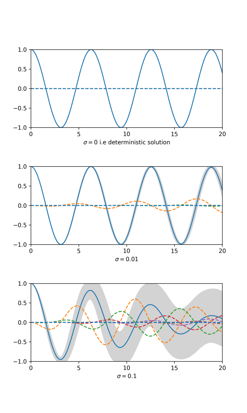
Stochastic Galerkin
Random ODE
Other formulations
Control formulation
Problem
Keywords/Mathematics
(Olson+2003), (Azouani+2011)
Nudging/Continuous Data Assimilation
Squeezing property, Determining mode/node
AOT-algorithm
If we have noiseless & continuous time observations
through an orthogonal projection
→ copy obs. to the simulated state
(true)
(simulate)
PDE (Partial Differential Equations)
Control theory/Synchronization
Incomplete atmospheric data
(Charney+1969)
copy
converge
Variational formulation
Problem
Keywords/Mathematics
(Law+2015), (Korn+2009)
4DVar
Adjoint method to compute gradient
Optimization, Iteration method
To estimate the initial state
from observation data
minimize a cost function.
Supervised Learning
Back propagation
DA & Numerical Analysis
Discretization/Model errors
Motivation
- Including discretization errors in the error analysis.
- Consider more general model errors and ML models.
- Error analysis with ML/surrogate models.
(Reich+2015)
Question
- Can we introduce the errors as random noises in models?
- Can minor modifications to the existing error analysis work?
Math: Numerical analysis, UQ
Dimension-reduction for dissipative dynamics
Motivation
- Defining "essential dimension" and relaxing the condition:
- should be independent of discretization.
(Tokman+2013)
Question
- Dissipativeness, dimension of the attractor?
- Does the dimension depend on time and state? (hetero chaos)
- Related to the SVD and the low-rank approximation?
Attractor
Math: Dynamical system
Numerics for UQ
Motivation
- Computing the Lyapunov spectrum of atmospheric models.
- Estimating unstable modes (e.g., singular vectors of Jacobian).
(Bridges+2001) (Ginelli+2007) (Saiki+2010)
Question
- Can we approximate them only using ensemble simulations?
- Can we estimate their approximation errors?

Math: Lyapunov analysis, Numerical analysis
Imbalance problems
Motivation
- Assimilating observations can break the balance relations inherited from dynamics. → numerical divergence
(e.g., geostrophic balance and gravity waves)
- Explaining the mechanism (sparsity or noise of observations?).
- Only ad hoc remedies (Initialization, IAU).
|
(Kalney 2003), (Hastermann+2021) |
Question
- Need to define a space of balanced states?
- Need to discuss the analysis state belonging to the space?
- Can we utilize structure-preserving schemes?
balanced states
Math: Structure-preserving scheme, constrained optimization
Related topics
Stochastic Galerkin
Problem
Keywords/Mathematics
(Sullivan2015) (Janjić+2023)
Weak formulation, Galerkin method, Lax-Milgram,
Generalized Polynomial Chaos Expansions
Karhunen–Lo`eve Expansions
Spectral expansion for sample space.

Random field
is represented by
using a stochastic germ
and the associated polynomials
We can compute cumulants using the coefs.
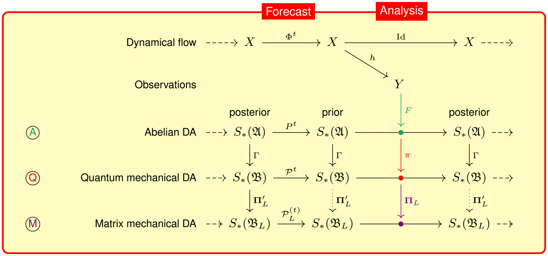
Quantum DA & Operator Algebra
Problem
Keywords/Mathematics

Koopman operator
Generalizing data assimilation by embedding it in a nonabelian operator algebra based on von Neuman algebra
Quantum mechanics
Quantum computer
Observable
Embedding
State
continuous linear positive functionals on
Metrics on DA
Problem
Keywords/Mathematics
Persistent Homology
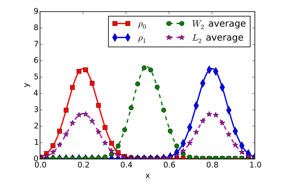
In the variational formulation, the analysis state can be understood as the barycenter of the prediction and observation.
(N. Feyeux et al. 2018)

Signature / Rough path
Wasserstein / OT
(N. Feyeux et al. 2018)
Different ways to define a barycenter.
Limitation of the Euclid average.
PF & Optimal Transport
Problem
Keywords/Mathematics
(Reich2013)
Optimal Transport, Sinkhorn algorithm
Monge-Kantorovich, Benamou-Brenier
prior
posterior
Aim: obtain equal-weighted posterior samples
OT
Gradient flow
Mean-field, Fokker-Planck
Diffusion model
Schrödinger bridge
stochastic-ver.
Prior samples
Seek a coupling
between two discrete random variables
(Jarrah+2023)
Mathematical analysis of data assimilation and related topics
By kotatakeda
Mathematical analysis of data assimilation and related topics
Applied Mathematics Freshman Seminar 2024 Kyoto
- 577


