Error Analysis of
the Ensemble Square Root Filter for Dissipative Dynamical Systems
2025/01/23 @Kyoto University
Supervisors
Professor Takashi Sakajo, Kyoto University
Professor Takemasa Miyoshi, Kyoto University & RIKEN
Professor Sebastian Reich, University of Potsdam
Kota Takeda
*
Department of mathematics, Kyoto University
*

Introduction
Setup
Bayesian filtering
Algorithms
Results (Error analysis)
Existing results for EnKF
My results
Summary & Discussion
Contents
Related sections in Thesis
Section 1, 2, 5
Section 3
Section 4
Section 6
Section 7
Section 8
Data Assimilation (DA)
The seamless integration of data and models
Model
Dynamical systems and its numerical simulations
ODE, PDE, SDE,
Numerical analysis, HPC,
Fluid mechanics, Physics
chaos
error
Data
Obtained from experiments or measurements
Statistics, Data analysis,
Radiosonde/Radar/Satellite observation
noise
limited
×


\partial_t \bm{u} + (\bm{u} \cdot \nabla) \bm{u} = - \frac{1}{\rho} \nabla p + \nu \triangle \bm{u} + \bm{f}

Each has uncertainty! (incomplete)
Numerical Weather Prediction (NWP)
Numerical Weather Prediction (NWP) uses atmospheric models
→ Unpredictable in long-term

Typhoon route circles

\partial_t \bm{u} + (\bm{u} \cdot \nabla) \bm{u} = - \frac{1}{\rho} \nabla p + \nu \triangle \bm{u} + \bm{f} \text{ \& } \dots
A small initial error can
grow exponentially fast.
state


time
true/nature state
simulated state
→ Chaotic
NWP and DA
→ chaotic
→ unpredictable in long-term
Numerical Weather Prediction (NWP) uses atmospheric models
Data Assimilation (DA):
simulate
true state
prediction
\widehat{v}_n
v_{n-1}
u_{n-1}
(not accessible directly)
u_n
Atmospheric
model
observation
y_n
Correct using observations (noisy, partial)
Correct using
v_n
indirect information from the true state
\widehat{v}_n
\partial_t \bm{u} + (\bm{u} \cdot \nabla) \bm{u} = - \frac{1}{\rho} \nabla p + \nu \triangle \bm{u} + \bm{f}
time
t_{n-1}
t_n
NWP & DA
in DA for Numerical Weather Prediction:
chaotic
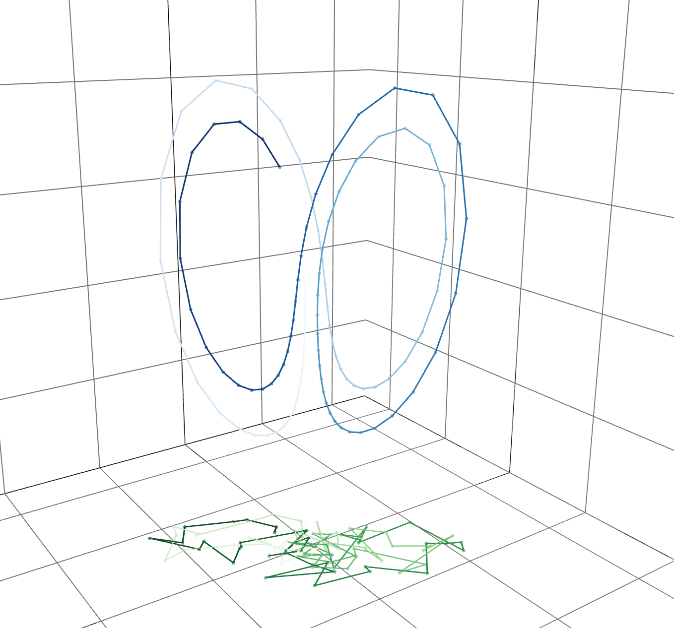
(x,y,z)\mapsto(x,y)
noisy
partial
observation
true state
\mathbb{R}^3
Example: the trajectory of the Lorenz 63 equation and observations.
Estimating the time series of states of
chaotic dynamical system
using noisy and partial observations.
Three difficulties
Considered
in this talk
Not considered
in this talk
Data Assimilation (DA)
-
Control
- Nudging/Continuous Data Assimilation
-
Bayesian Filtering
- Particle Filter (PF)
- Ensemble Kalman filter (EnKF)
-
Variational
- Four-dimensional Variation method (4DVar)
Several formulations & algorithms of DA:
Focus on the main results
(T.+2024) & Thesis
Related to partial observations
cf. Section 5
Not covered
cf. Section 1
Mathematics on DA:
Functional analysis, Probability theory, Dynamical systems,
Partial differential equations, (Numerical analysis)
cf. Section 2, 5
Control formulation
Problem
Keywords/Mathematics
(Olson+2003), (Azouani+2011)
Nudging/Continuous Data Assimilation
Squeezing property, Determining mode/node
AOT-algorithm
\frac{du}{dt} = \mathcal{F}(u),
v = \mathcal{P} u + q, \quad \frac{dq}{dt} = (I - \mathcal{P})\mathcal{F}(v).
If we have noiseless & continuous time observations
through an orthogonal projection
→ copy obs. to the simulated state
(true)
(simulate)
\mathcal{P}: \mathcal{U} \rightarrow \mathcal{Y}.
\text{Estimate the smallest rank of } \mathcal{P} \text{ s.t.}
\lim_{t \rightarrow \infty}|v(t) -u(t)| \rightarrow 0.
PDE (Partial Differential Equations)
Control theory/Synchronization
Incomplete atmospheric data
(Charney+1969)
u = \sum_{|k| \le \lambda} u_k \phi_k + \sum_{|k| >\lambda} u_k \phi_k
v = \sum_{|k| \le \lambda} u_k\phi_k + \sum_{|k| >\lambda} v_k \phi_k
\mathcal{P}_{\lambda} u
copy
converge
(t\rightarrow\infty)
\lambda > 0: \text{ threshold for wavelength}
observed
unobserved
Variational formulation
Problem
Keywords/Mathematics
(Law+2015), (Korn+2009)
Four-dimensional Variational method (4DVar)
Adjoint method to compute gradient
Optimization, Iteration method
\text{Well-posedness of a mininization problem}
v_0 = \argmin_{u_0} J(u_0; \theta)
To estimate the initial state
from observation data
y_1, \cdots, y_N \in \mathcal{Y}
J(u_0;\theta) = \sum_{n=1}^N \|R^{-1/2} (y_n - h(\Psi_{\tau n}(u_0;\theta)))\|^2
u_0 \in \mathcal{U}
minimize a cost function.
\nabla_{u_0} J(u_0)
u_0
y_1
y_2
y_3
y_4
u_1
u_2
u_3
u_4
Supervised Learning
(\theta: \text{ model parameters})
\widehat{\theta} = \argmin_{\theta} J(u_0; \theta)
Back propagation
\text{Suppose } y_n \sim \mathcal{N}(h(u_n), R).
Introduction
Setup
Bayesian filtering
Algorithms
Results (Error analysis)
Existing results for EnKF
My results
Summary & Discussion
Contents
Related sections in Thesis
Section 1, 2, 5
Section 3
Section 4
Section 6
Section 7
Section 8
State estimation with chaos, noise
Setup: Model
\frac{d u}{dt} = \mathcal{F}(u)
(\mathcal{F}: \mathcal{U} \rightarrow \mathcal{U}, u(0) = u_0 \in \mathcal{U})
u(t) = \Psi_t (u_0)
Model dynamics in
Semi-group in
\mathcal{U}
\mathcal{U}
generates
\mathcal{U}
(\Psi_t : \mathcal{U} \rightarrow \mathcal{U}, t \ge 0)
(assume)
: separable Hilbert space
: separable Hilbert space (state space)
The known model generates
the unknown true trajectory.
t
unknown trajectory
unknown
See Section 3 for other formulations.
Setup: Observation
Discrete-time model (at obs. time)
\mathcal{U}
(\Psi = \Psi_\tau, \tau > 0 \text{: observation interval})
We have noisy observations in
t
y_n = H u_n + \eta_n, \ n \in \mathbb{N}.
(H: \mathcal{L}(\mathcal{U}, \mathcal{Y}), \eta_n \sim N(0, R))
Noisy observation
u_n = \Psi(u_{n-1})
observe
u_1
y_1
u_2
y_2
t_1
t_2
t_3
...
\tau
bounded linear
\in \mathcal{Y}
\mathcal{Y}
(another Hilbert space)
\in \mathcal{Y}
\Psi
at discrete time steps.
(6.4)
(6.2)
Sequential state estimation
\mathcal{U}
t
y_1
y_2
t_1
t_2
t_3
...
\tau
given
\bm{y}_n = \{y_i \mid i \le n\}
Problem
u_n
estimate
\text{For } n \in \mathbb{N},
known:
\Psi,
H,
obs. noise distribution.
y_2
y_3
u_1
u_2
u_3
\Psi
\Psi
Bayesian Data Assimilation
Approach: Bayesian Data Assimilation
\mathbb{P}^{v_n} = \mathbb{P}^{u_n}({}\cdot{} | \bm{y}_n).
→ construct a random variable so that
v_n
In other words, compute (approximate)
the conditional distribution .
\mathbb{P}^{u_n}({}\cdot{} | \bm{y}_n)
(filtering distribution)
given
\bm{y}_n = \{y_i \mid i \le n\}
Problem
u_n
Estimate
\text{※ } v_n \text{ should be adopted to the filtration } F_n = \sigma(\bm{y}_n).
Sequential Data Assimilation
\mathbb{P}^{v_{n-1}}
y_n
\mathcal{U}

y_n
y_{n+1}
t
t_{n-1}
t_n
t_{n+1}
\tau
For n, two steps with auxiliary variable .
\hat{v}_n
\Rightarrow \mathbb{P}^{v_n} = \mathbb{P}^{u_n}({}\cdot{} | \bm{y}_n).
Proposition
\text{Assume } \mathbb{P}^{v_0} = \mathbb{P}^{u_0}.
The n-iterations (I) & (II)
Decomposition into the iterative algorithm
Definition 3.7, 10

(I) Prediction
\Psi
(I) Prediction
\mathbb{P}^{\hat{v}_n}
by model
(II)Analysis
(II) Analysis
\mathbb{P}^{v_n}
by Bayes' rule
\mathbb{P}^{v_n} \propto L_{y_n} \cdot \mathbb{P}^{\hat{v}_n}
likelihood function
Prediction
...
Repeat (I) & (II)
Introduction
Setup
Bayesian filtering
Algorithms
Results (Error analysis)
Existing results for EnKF
My results
Summary & Discussion
Contents
Related sections in Thesis
Section 1, 2, 5
Section 3
Section 4
Section 6
Section 7
Section 8
State estimation with chaos, noise.
Compute
\mathbb{P}^{u_n}({}\cdot{} | \bm{y}_n).
Filtering algorithms
Only focus on the Gaussian-based Algorithms
Many filtering algorithms
PF
Ensemble based
EnKF
"Gaussian based"
KF
KF & EnKF
Kalman filter (KF) [Kalman 1960]
- All Gaussian distribution
- Closed update of mean and covariance.
Assume: linear F, Gaussian noises
\mathbb{P}^{v_n} = \mathcal{N}(\varpi_n, P_n).
\mathbb{P}^{v_n} \approx \frac{1}{m} \sum_{k=1}^m \delta_{v_n^{(k)}}.
Ensemble Kalman filter (EnKF)
Non-linear extension by Monte Carlo method
- Update of ensemble
V_n = [v_n^{(1)},\dots,v_n^{(m)}] \in \mathcal{U}^m
(Reich+2015) S. Reich and C. Cotter (2015), Probabilistic Forecasting and Bayesian Data Assimilation, Cambridge University Press, Cambridge.
(Law+2015) K. J. H. Law, A. M. Stuart, and K. C. Zygalakis (2015), Data Assimilation: A Mathematical Introduction, Springer.
KF & EnKF
Kalman filter(KF)
Assume: linear F, Gaussian noises
\varpi_n, P_n
\widehat{\varpi}_n, \widehat{P}_n
\varpi_{n-1}, P_{n-1}
y_n
Linear F
Bayes' rule
predict
analysis
Ensemble Kalman filter (EnKF)
Non-linear extension by Monte Carlo method
V_n
V_{n-1}
\widehat{V}_n
y_n
V_n = [v_n^{(k)}]_{k=1}^m, \widehat{V}_n = [\widehat{v}_n^{(k)}]_{k=1}^m.
\text{nonlinear } \mathcal{F}
\widehat{\varpi}_n, \widehat{P}_n
\varpi_n, P_n
approx.
ensemble
\approx
\approx
\varpi_n \approx \overline{v}_n = \frac{1}{m} \sum_{k=1}^m v^{(k)}_n
P_n = \operatorname{Cov}_m(V_n) = \frac{1}{m-1} \sum_{k=1}^m (v^{(k)}_n - \overline{v}_n) \otimes (v^{(k)}_n - \overline{v}_n)
Two variants
→ next slide
Definition 4.1
- Two major variants of EnKF:
- Perturbed Observation (PO): stochastic → sampling error
- Ensemble Transform Kalman Filter (ETKF): deterministic
Two EnKF variants
\mathcal{U}
t
y_1
y_2
t_1
t_2
t_3
...
\tau
t_0
Repeat (I) & (II)
(II)Analysis
(I) Prediction
\Psi
v_0^{(1)}
v_0^{(m)}
v_0^{(2)}


\widehat{v}_1^{(1)}
v_1^{(1)}
\vdots
(Burgers+1998)
(Bishop+2001)
PO (stochastic EnKF)
\widehat{v}^{(k)}_n = \Psi(v^{(k)}_{n-1}), \quad k = 1, \dots, m.
(I) V_{n-1} \rightarrow \widehat{V}_n: \text{ Evolve each member by model dynamics } \Psi,
(Burgers+1998) G. Burgers, P. J. van Leeuwen, and G. Evensen (1998), Analysis Scheme in the Ensemble Kalman Filter, Mon. Weather Rev., 126, 1719–1724.
Stochastic!
Perturbed Observation
\cdot^\top
: A transpose (adjoint) of a matrix (linear operator)
Definition 4.10
y^{(k)}_n = y_n + \eta_n^{(k)}, \quad \eta_n^{(k)} \sim N(0, R), \quad k = 1, \dots, m.
(II) \widehat{V}_n, y_n \rightarrow V_n: \text{Replicate observations,}\\
\text{Then, update each member,}
(\bigstar)
v_n^{(k)} = (I - K_n H) \widehat{v}_n^{(k)} + K_n y_n^{(k)}, \quad k = 1, \dots, m,
\text{where } K_n = \widehat{P}_n H^\top (H \widehat{P}_n H^\top + R)^{-1}, \widehat{P}_n = \operatorname{Cov}_m(\widehat{V}_n).
ETKF (deterministic EnKF)
\widehat{v}^{(k)}_n = \Psi(v^{(k)}_{n-1}), \quad k = 1, \dots, m.
(I) V_{n-1} \rightarrow \widehat{V}_n: \text{ Evolve each member by model dynamics } \Psi,
(Bishop+2001) C. H. Bishop, B. J. Etherton, and S. J. Majumdar (2001), Adaptive Sampling with the Ensemble Transform Kalman Filter. Part I: Theoretical Aspects, Mon. Weather Rev., 129, 420–436.
Deterministic!
\text{with the transform matrix } T_n \in \mathbb{R}^{m \times m} \text{ s.t. }
(II) \widehat{V}_n, y_n \rightarrow V_n: \text{Decompose } \widehat{V}_n =\overline{\widehat{v}}_n + d\widehat{V}_n.\\
\overline{v}_n = (I - K_n H)\overline{\widehat{v}}_n + K_n y_n , \quad dV_n = d\widehat{V}_n T_n.
\text{Then, update separately,}
\frac{1}{m-1} d\widehat{V}_n T_n (d\widehat{V}_n T_n)^\top = (I - K_n H) \widehat{P}_n
The explicit representation exists!
(\bigstar)
Ensemble Transform Kalman Filter
Definition 4.13
ETKF (deterministic EnKF)
Ensemble Transform Kalman Filter
\text{The transform matrix } T_n \in \mathbb{R}^{m \times m} \text{ satisfying}
\frac{1}{m-1} d\widehat{V}_n T_n (d\widehat{V}_n T_n)^\top = (I - K_n H) \widehat{P}_n
Lemma (Theorem 4.1)
\text{is uniquely given by}
T_n = \left(I+ \frac{1}{m-1} d\widehat{V}_n^\top H^\top R^{-1} H d\widehat{V}_n \right)^{-\frac{1}{2}}.
\text{(up to unitary transformation)}
ETKF is one of the deterministic EnKF algorithms known as ESRF (Ensemble Square Root Filters).
※ESRF (deterministic EnKF)
ESRF
ETKF
\frac{1}{m-1} d\widehat{V}_n T_n (d\widehat{V}_n T_n)^\top = (I - K_n H) \widehat{P}_n.
T_n \in \mathbb{R}^{m \times m}
EAKF (Ensemble Adjustment Kalman Filter)
\frac{1}{m-1} A_n d\widehat{V}_n (A_n d\widehat{V}_n)^\top = (I - K_n H) \widehat{P}_n.
A_n \in \mathcal{L}(\mathcal{U})
: bounded linear
(Anderson 2001) J. L. Anderson (2001), An Ensemble Adjustment Kalman Filter for Data Assimilation, Mon. Weather Rev., 129, 2884–2903.
Key perspective of EnKF (KF)
v_n = (I - K_n H) \widehat{v}_n + K_n y_n,
(\bigstar)
\text{where } K_n = \widehat{P}_n H^\top (H \widehat{P}_n H^\top + R)^{-1}.
The analysis state is the weighted average of
the prediction and observation
v_n
\widehat{v}_n
y_n
The weight is determined by estimated uncertainties
K_n
R
: uncertainty in observation (prescribed)
\widehat{P}_n
: uncertainty in prediction (approx. by ensemble)
Inflation (numerical technique)
Issue: Underestimation of covariance through the DA cycle
→ Overconfident in the prediction → Poor state estimation
(I) Prediction → inflation → (II) Analysis → ...
Rank is improved
Rank is not improved
\widehat{P}_n
Idea: inflating the covariance before (II)
Two basic methods of inflation
\text{Additive } (\alpha \ge 0)
\text{Multiplicative } (\alpha \ge 1)
\text{ETKF}: d\widehat{V}_n \rightarrow \alpha d\widehat{V}_n.
\text{where } d\widehat{V}_n = [\widehat{v}^{(k)}_n - \overline{\widehat{v}}_n]_{k=1}^m, \overline{\widehat{v}}_n = \frac{1}{m} \sum_{k=1}^m \widehat{v}^{(k)}_n.
\text{PO}: \widehat{P}_n \rightarrow \alpha^2\widehat{P}_n,
\text{Only for PO}: \widehat{P}_n \rightarrow \widehat{P}_n + \alpha^2 I_{\mathcal{U}}.
※depending on the implementation
※
Section 4.4
PO
Two EnKF variants
Simple
Stochastic
Require many samples
ETKF
Complicated
Deterministic
Require few samples
Practical !
Inflation: add., multi.
Inflation: only multi.
※depending on the implementation
※
Filtering algorithms
Many filtering algorithms
PF
Ensemble based
EnKF
"Gaussian based"
KF
Deterministic
Stochastic
PO
ETKF
EAKF
Introduction
Setup
Bayesian filtering
Algorithms
Results (Error analysis)
Existing results for EnKF
My results
Summary & Discussion
Contents
Related sections in Thesis
Section 1, 2, 5
Section 3
Section 4
Section 6
Section 7
Section 8
State estimation with chaos, noise.
Compute
\mathbb{P}^{u_n}({}\cdot{} | \bm{y}_n).
EnKF: Ensemble & Gaussian approximation.
Error analysis of EnKF
Assumptions on model
(Reasonable)
Assumption on observation
(Strong)
We focus on finite-dimensional state spaces
(\mathcal{U} = \R^{N_u} \text{ for } N_u \in \mathbb{N})
(T.+2024) K. T. & T. Sakajo (2024), SIAM/ASA Journal on Uncertainty Quantification, 12(4), 1315–1335.
Assumptions for analysis
N_y = N_u, H = I_{N_u}, \eta \sim \mathcal{N}(0, r^2 I_{N_u}), r > 0.
Assumption (obs-1)
"full observation"
Strong!
\exist \rho > 0 \text{ s.t. } \forall u_0 \in B(\rho), \forall t > 0, u(t ; u_0) \in B(\rho).
\exist \beta > 0 \text{ s.t. } \forall u \in B(\rho), \forall v \in \mathbb{R}^{N_u},
\langle F(u) - F(v), u - v \rangle \le \beta | u - v|^2.
\exist \beta > 0 \text{ s.t. } \forall u, v \in B(\rho), |F(u) - F(v)| \le \beta |u - v|.
Assumption (model-1)
Assumption (model-2)
Assumption (model-2')
\forall u_0 \in \R^{N_u}, \frac{du}{dt}(t) = F(u(t)) \text{ has an unique solution, and}
Reasonable
(B(\rho) = \{u \in \R^{N_u} \mid |u| \le \rho \})
"one-sided Lipschitz"
"Lipschitz"
"bounded"
or
Dissipative dynamical system
Dissipative dynamical system
Section 3, 5
Dissipative dynamical systems
Lorenz 63, 96 equations, widely used in geophysics,
\frac{du^i}{dt} = (u^{i+1} - u^{i-2}) u^{i-1} - u^i + f \quad (i = 1, \dots, N_u),
Example (Lorenz 96)
\bm{u} = (u^i)_{i=1}^{N_u} \in \mathbb{R}^{N_u}, f \in \R,
non-linear conserving
linear dissipating
forcing
Assumptions (model-1, 2, 2')
hold
incompressible 2D Navier-Stokes equations (2D-NSE) in infinite-dim. setting
Lorenz 63 eq. can be written in the same form.
→ We can discuss ODE and PDE in a unified framework.
can be generalized
\frac{du}{dt} =
B(u, u)
+
A u
+
f.
bilinear operator
linear operator
dissipative dynamical systems
Mimics chaotic variation of
physical quantities at equal latitudes.
(Lorenz1996) (Lorenz+1998)
u
Dissipative dynamical systems
The orbits of the Lorenz 63 equation.
Literature review
-
Consistency (Mandel+2011, Kwiatkowski+2015)
-
Sampling errors (Al-Ghattas+2024)
-
Stability (Tong+2016a,b)
-
Error analysis (full observation )
-
PO + add. inflation (Kelly+2014) → next slide
-
ETKF + multi. inflation (T.+2024) → current
-
EAKF + multi. inflation (T.)
-
-
Error analysis (partial observation) → future (partially solved, T.)
H = I_{N_u}
How EnKF approximate KF?
How EnKF approximate
the true state?
※ Continuous time formulation (EnKBF)
-
EnKBF with full-obs. (de Wiljes+2018)
Section 6
(m \rightarrow \infty)
Error analysis of PO (prev.)
\text{Let us consider the PO method with additive inflation } \alpha > 0.
\text{Let } e^{(k)}_n = v^{(k)}_n - u_n \text{ for } k = 1, \dots, m.
(Kelly+2014) D. Kelly et al. (2014), Nonlinearity, 27(10), 2579–2603.
\widehat{P}_n \rightarrow \widehat{P}_n + \alpha^2 I_{N_u}
Strong effect! (improve rank)
Theorem (Kelly+2014)
\mathbb{E} [|e^{(k)}_n|^2] \le \theta^n \mathbb{E} [|e^{(k)}_0|^2] + 2m r^2 \frac{1 - \theta^n}{1-\theta}
\text{Then, } \exist \theta = \theta(\beta, \tau, r, \alpha) \in (0, 1), \text{ s.t. }
\text{Let Assumptions (obs-1, model-1,2) hold and }\alpha \gg 1.
\text{for } n \in \mathbb{N}, k = 1, \dots, m.
exponential decay
initial error
\mathbb{E} [\cdot] \text{ : expectation w.r.t. obs. noise and initial uncertainty}
Error analysis of PO (prev.)
\text{Let us consider the PO method with additive inflation } \alpha > 0.
\text{Let } e^{(k)}_n = v^{(k)}_n - u_n \text{ for } k = 1, \dots, m.
variance of observation noise
uniformly in time
(Kelly+2014) D. Kelly et al. (2014), Nonlinearity, 27(10), 2579–2603.
\widehat{P}_n \rightarrow \widehat{P}_n + \alpha^2 I_{N_u}
Strong effect! (improve rank)
Corollary (Kelly+2014)
\limsup_{n \rightarrow \infty} \mathbb{E} [|e^{(k)}_n|^2] \le \frac{2 m}{1-\theta}r^2
\text{Then, } \exist \theta = \theta(\beta, \tau, r, \alpha) \in (0, 1), \text{ s.t. }
\text{Let Assumptions (obs-1, model-1,2) hold and }\alpha \gg 1.
\text{for } k = 1, \dots, m.
\mathbb{E} [\cdot] \text{ : expectation w.r.t. obs. noise and initial uncertainty}
Introduction
Setup
Bayesian filtering
Algorithms
Results (Error analysis)
Existing results for EnKF
My results
Summary & Discussion
Contents
Related sections in Thesis
Section 1, 2, 5
Section 3
Section 4
Section 6
Section 7
Section 8
State estimation with chaos, noise.
Compute
\mathbb{P}^{u_n}({}\cdot{} | \bm{y}_n).
EnKF: Ensemble & Gaussian approximation.
PO+add. infl. (Kelly+2014)
Error analysis of ETKF (our)
\text{Let } e_n =\overline{v}_n - u_n \text{ where } \overline{v}_n = \frac{1}{m} \sum_{k=1}^m v^{(k)}_n.
\text{Let us consider the ETKF with multiplicative inflation } \alpha \ge 1.
(T.+2024) K. T. & T. Sakajo (2024), SIAM/ASA Journal on Uncertainty Quantification, 12(4), 1315–1335.
\mathbb{E}[|e_n|^2] \le \theta^n \mathbb{E}[|e_0|^2] + \frac{N_u r^2(1 - \theta^n)}{1-\theta} + \left(\frac{1 - \Theta}{1 - \theta} - 1\right)D.
Theorem 7.3 (T.+2024)
\text{where } \Theta = \Theta(\beta, \rho, \tau, r, m, \alpha) , D = D(\beta, \rho) > 0.
\text{Then, } \exist \theta = \theta(\beta, \rho, \tau, r, m, \alpha) < 1\text{ s.t.}
\text{Let Assumptions (obs-1, model-1,2') hold.}
\text{Suppose } m > N_u, \operatorname{rank}(P_0) = N_u,\alpha \gg 1, \text{ and}
v_n^{(k)} \in B(\rho) \text{ for } k = 1, \dots, m \text{ and } n \in \N.
※ The same result holds for the EAKF (Theisis)
Error analysis of ETKF (our)
\text{Let us consider the ETKF with multiplicative inflation } \alpha \ge 1.
(T.+2024) K. T. & T. Sakajo (2024), SIAM/ASA Journal on Uncertainty Quantification, 12(4), 1315–1335.
\limsup_{n \rightarrow \infty} \mathbb{E}[|e_n|^2] \le \frac{N_u r^2}{1-\theta} + \left(\frac{1 - \Theta}{1 - \theta} - 1\right)D.
Corollary 7.3 (T.+2024)
\text{where } \Theta = \Theta(\beta, \rho, \tau, r, m, \alpha) , D = D(\beta, \rho) > 0.
\text{Then, } \exist \theta = \theta(\beta, \rho, \tau, r, m, \alpha) < 1\text{ s.t.}
\text{Let Assumptions (obs-1, model-1,2') hold.}
\text{Suppose } m > N_u, \operatorname{rank}(P_0) = N_u,\alpha \gg 1, \text{ and}
v_n^{(k)} \in B(\rho) \text{ for } k = 1, \dots, m \text{ and } n \in \N.
\text{Let } e_n =\overline{v}_n - u_n \text{ where } \overline{v}_n = \frac{1}{m} \sum_{k=1}^m v^{(k)}_n.
Sketch: Error analysis of ETKF (our)
< e^{-\beta \tau}
= \frac{1}{1 + \alpha^2 r^{-2} \lambda_{min}(\widehat{P}_n)}
①
②
Key point!
\because
(1) \text{ We establish a lower bound of eigenvalues of } \widehat{P}_n \text{ by } \alpha \gg 1.
(2) \text{ If } \widehat{P}_n \text{ is positive-difinite, we have a bound by } \alpha \gg 1.
e^{\beta \tau}
Error growth at (I)
\|(I + \alpha^2 r^{-2} \widehat{P}_n)^{-1}\|_{op}
Error contraction at (II)
norm of error
t
Sketch: Error analysis of ETKF (our)
Strategy: estimate the changes in DA cycle
\widehat{e}_n
(\widehat{e}_n = \overline{\widehat{v}}_n - u_n)
(I)
(II)
expanded
by dynamics
contract &
noise added
e_{n-1}
e_n
Applying Gronwall's lemma to the model dynamics,
(I)
| \widehat{e}_n | \le e^{\beta \tau} |e_{n-1}|
+ {additional term}.
①
\overline{v}_n = (I - K_n H)\overline{\widehat{v}}_n + K_n y_n
e_n = (I - K_n H) \widehat{e}_n + K_n (y_n - H u_n).
subtracting yields
(II)
From the Kalman update relation
(\bigstar)
u_n
prediction error
② contraction
③ obs. noise effect
estimated by op.-norm
Sketch: Error analysis of ETKF (our)
Key estimates in
Using Woodbury's lemma, we have
I - K_n H = (I + \widehat{P}_n H^\top R^{-1} H)^{-1}.
② contraction
③ obs. noise
(II)
\| \cdot \|_{op}: \text{operator norm}
\|I - K_n H\|_{op} = \|(I + \widehat{P}_n H^\top R^{-1} H)^{-1}\|_{op}
Contraction (see the next slide)
= \|(I + \alpha^2 r^{-2}\widehat{P}_n)^{-1}\|_{op}.
H = I, R = r^2 I
assumption
\|K_n\|_{op} = \|(I + \alpha^2 r^{-2}\widehat{P}_n)^{-1} \alpha^2 r^{-2}\widehat{P}_n\|_{op} \le 1.
(\forall \alpha, r \ge 0, \widehat{P}_n \text{: positive-definite})
Sketch: Error analysis of ETKF (our)
\text{Let } \widehat{\lambda}_n = \lambda_{min}(\widehat{P}_n), \lambda_n = \lambda_{min}(P_n).
(1) \text{ We establish a lower bound of eigenvalues of } \widehat{P}_n \text{ by } \alpha \gg 1.
\widehat{\lambda}_{n-1} \rightarrow \lambda_n \rightarrow \widehat{\lambda}_n
\Rightarrow \widehat{\lambda}_n \ge \frac{e^{-c\tau} \alpha^2 \widehat{\lambda}_{n-1}}{1 + \alpha^2 r^{-2} \widehat{\lambda}_{n-1}}
\therefore \liminf_{n \rightarrow \infty} \widehat{\lambda}_n \ge \frac{r^2 (e^{-c\tau} \alpha^2 - 1)}{\alpha^2} > 0.
estimate the change
\widehat{\lambda}_{n-1} \rightarrow \lambda_n
(inflation & analysis)
\lambda_n = \frac{\alpha^2 \widehat{\lambda}_{n-1}}{1 + \alpha^2 r^{-2} \widehat{\lambda}_{n-1}}
\lambda_n \rightarrow \widehat{\lambda}_n
(prediction)
\widehat{\lambda}_n \ge e^{-c\tau} \lambda_n
\left(c = \frac{8m \beta\rho^2}{m-1}\right)
Comparison
\limsup_{n \rightarrow \infty} \mathbb{E}[|e^{(k)}_n|^2] \le \frac{2 m}{1-\theta}r^2,
\limsup_{n \rightarrow \infty} \mathbb{E}[|e_n|^2] \le \frac{N_u r^2}{1-\theta} + \left(\frac{1 - \Theta}{1 - \theta} - 1\right)D.
\text{Suppose } m > N_u \text{ and } \alpha \gg 1,
\text{Suppose } \alpha \gg 1,
ETKF with multiplicative inflation (our)
PO with additive inflation (prev.)
= O(r^2)
r \rightarrow 0
accurate observation limit
= O(r^2)
O(r^4)
\text{for } k = 1, \dots, m.
Two Gaussian-based filters (EnKF) are assessed in terms of the state estimation error.
due to
due to
Numerical results
Observing System Simulation Experiment (OSSE)
A standard numerical test framework for DA algorithms.
Numerical results
Observing System Simulation Experiment (OSSE)
t
t_1
t_2
t_3
\tau
u_1
u_2
u_3
(1) Compute the true solution to (6.2).
u_n
\mathcal{U}
Numerical results
Observing System Simulation Experiment (OSSE)
t
t_1
t_2
t_3
\tau
u_1
u_2
u_3
(2) Generate random observations as in (6.4).
y_n
(1) Compute the true solution to (6.2).
u_n
\mathcal{U}
y_1
y_2
y_3
Numerical results
Observing System Simulation Experiment (OSSE)
t
t_1
t_2
t_3
\tau
v_n
(3) Assimilate the observed data and obtain the analysis states using a data assimilation algorithm.
y_n
(2) Generate random observations as in (6.4).
y_n
(1) Compute the true solution to (6.2).
u_n
\mathcal{U}
v_1
v_2
v_3
y_1
y_2
y_3
DA algorithm
Numerical results
Observing System Simulation Experiment (OSSE)
t
t_1
t_2
t_3
\tau
(2) Generate random observations as in (6.4).
y_n
(1) Compute the true solution to (6.2).
u_n
\mathcal{U}
v_1
v_2
v_3
(3) Assimilate the observed data and obtain the analysis states using a data assimilation algorithm.
y_n
v_n
(4) Compute the error between and for n = 1, 2, ...
u_n
v_n
e_1
e_2
e_3
u_1
u_2
u_3
Numerical results
OSSE: ETKF for the Lorenz 96 equation
N_u = 40, m = N_u+1 = 41, r = 1.0.
SE = \mathbb{E}[|e_n|^2]
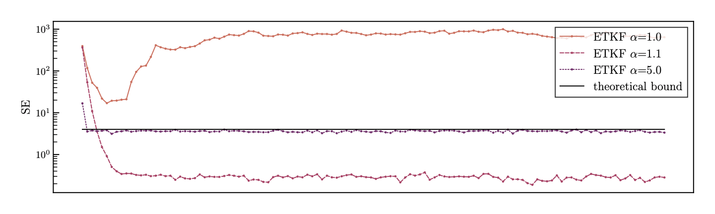
n
\le N_u r^2 + ...
From Theorem 7.3
→ theoretical bound
(\text{Suppose } \theta \ll 1)
strong inflation
weak inflation
no inflation
Numerical results

O(r^2)
Dependency on observation noise variance .
r^2
Numerical results
Animation
Introduction
Setup
Bayesian filtering
Algorithms
Results (Error analysis)
Existing results for EnKF
My results
Summary & Discussion
Contents
Related sections in Thesis
Section 1, 2, 5
Section 3
Section 4
Section 6
Section 7
Section 8
State estimation with chaos, noise.
Compute
\mathbb{P}^{u_n}({}\cdot{} | \bm{y}_n).
EnKF: Ensemble & Gaussian approximation.
PO+add. infl. (Kelly+2014)
ESRF+multi. infl. (T.+2024)
Summary
We focus on
The sequential state estimation using model and data.
Results
Error analysis of a practical DA algorithm (ETKF)
under an ideal setting (T.+2024).
Discussion
Two issues with extending our analysis.
→ should be relaxed in the future
(rank deficient, non-symmetric)
Discussion
Current
(T.+2024)
1. Partial observation
2. Small ensemble
m \le N_u
N_y < N_u, H \in \mathbb{R}^{N_y \times N_u}
3. Infinite-dimension
\text{state space } \mathcal{U}: \text{Hilbert space},
\text{observation space } \mathcal{Y} \subset \mathcal{U}.
partially solved (T.)
extend
Future
→ Issue 1, 2
→ Issue 1
→ Issue 1
Issues:
- rank deficient
- non-symmetric
Discussion
\|(I + \widehat{P}_n H^\top R^{-1} H)^{-1}\|_{op} \ge 1.
\text{If } m \le N_u \text{ or } N_y < N_u, H \in \mathbb{R}^{N_y \times N_u}, R \in \mathbb{R}^{N_y \times N_y},
Issue 1 (rank deficient)
\text{then,}
② Error contraction in (II)
1. Partial observation
2. Small ensemble
Discussion
\|(I + \widehat{P}_n H^\top R^{-1} H)^{-1} \widehat{P}_n H^\top R^{-1} H\|_{op} \le 1.
\text{Let } N_y < N_u, H \in \mathbb{R}^{N_y \times N_u}, R \in \mathbb{R}^{N_y \times N_y}.
Issue 2 (non-symmetric)
\text{If } \widehat{P}_n H^\top R^{-1} H \text{ is symmetric then,}
③ bound of obs. noise
If non-symmetric, it doesn't hold in general.
Example
A = \left[
\begin{array}{cc}
a & 0 \\
b & 0
\end{array}
\right]
\Rightarrow
\|(I + A)^{-1} A\|_{op} = \frac{\sqrt{a^2 + b^2}}{1+a} > 1.
(a > 0, b^2 \ge 1 + 2a)
Discussion
Infinite-dimension
Theorem (Kelly+2014) for PO + add. infl.
Theorem (T.+2024) for ETKF + multi. infl.
\text{state space } \mathcal{U}: \text{Hilbert space},
\text{observation space } \mathcal{Y} \subset \mathcal{U} \text{: Hilbert space}.
doesn't hold
(due to Issue 1: rank deficient)
※with full-observations
(ex: 2D-NSE with the Sobolev space)
( improve rank)
\because
still holds
Summary
I focus on
Sequential state estimation using model and data.
Results
Error analysis of a practical DA algorithm (ETKF)
under an ideal setting (T.+2024).
Discussion
Two issues with extending our analysis.
→ should be relaxed
(rank deficient, non-symmetric)
→ other problems in the future
Future Plans
NWP /
Fluid Mechanics
Thesis
DA
UQ
UQ (Uncertainty Quantification):
The quantitative studies of uncertainties in the real world applications.
Mathematics:
Functional analysis
Gronwall's inequality
Future Plans
NWP /
Fluid Mechanics
Thesis
DA
UQ
Collaborating with
Numerics, Machine Learning
Contributing to NWP
Continuing
Developing
novel algorithms
Other applications
Mathematics:
Functional analysis
Gronwall's inequality
Numerical analysis
Lyapunov analyis
Large deviations
Operator algebra
Computational topology
...
UQ (Uncertainty Quantification):
The quantitative studies of uncertainties in the real world applications.
Data Assimilation (DA)
-
Control
- Nudging/Continuous Data Assimilation
-
Bayesian
- Particle Filter (PF)
- Ensemble Kalman filter (EnKF)
-
Variational
- Four-dimensional Variation method (4DVar)
PDE
Machine
Learning
Back Prop.
Supervised Learning
Optimization
Dynamical system
SDE
Dynamics
Uncertainty Quantification
Probability/Statistics
& related topic
Random ODE
Numerical Analysis
structure-preserving
Numerical error
Lyapunov
analysis
Operator Algebra
Koopman operator
Quantum DA
Optimal Transport
Diffusion AI
Future plan
References
- (T.+2024) K. T. & T. Sakajo, SIAM/ASA Journal on Uncertainty Quantification, 12(4), 1315–1335.
- (T.) Kota Takeda, Error Analysis of the Ensemble Square Root Filter for Dissipative Dynamical Systems, PhD Thesis, Kyoto University, 2025.
- (Kelly+2014) D. T. B. Kelly, K. J. H. Law, and A. M. Stuart (2014), Well-posedness and accuracy of the ensemble Kalman filter in discrete and continuous time, Nonlinearity, 27, pp. 2579–260.
- (Al-Ghattas+2024) O. Al-Ghattas and D. Sanz-Alonso (2024), Non-asymptotic analysis of ensemble Kalman updates: Effective dimension and localization, Information and Inference: A Journal of the IMA, 13.
- (Tong+2016a) X. T. Tong, A. J. Majda, and D. Kelly (2016), Nonlinear stability and ergodicity of ensemble based Kalman filters, Nonlinearity, 29, pp. 657–691.
- (Tong+2016b) X. T. Tong, A. J. Majda, and D. Kelly (2016), Nonlinear stability of the ensemble Kalman filter with adaptive covariance inflation, Comm. Math. Sci., 14, pp. 1283–1313.
- (Kwiatkowski+2015) E. Kwiatkowski and J. Mandel (2015), Convergence of the square root ensemble Kalman filter in the large ensemble limit, Siam-Asa J. Uncertain. Quantif., 3, pp. 1–17.
- (Mandel+2011) J. Mandel, L. Cobb, and J. D. Beezley (2011), On the convergence of the ensemble Kalman filter, Appl.739 Math., 56, pp. 533–541.
References
-
(de Wiljes+2018) J. de Wiljes, S. Reich, and W. Stannat (2018), Long-Time Stability and Accuracy of the Ensemble Kalman-Bucy Filter for Fully Observed Processes and Small Measurement Noise, Siam J. Appl. Dyn. Syst., 17, pp. 1152–1181.
-
(Burgers+1998) G. Burgers, P. J. van Leeuwen, and G. Evensen (1998), Analysis Scheme in the Ensemble Kalman Filter, Mon. Weather Rev., 126, 1719–1724.
-
(Bishop+2001) C. H. Bishop, B. J. Etherton, and S. J. Majumdar (2001), Adaptive Sampling with the Ensemble Transform Kalman Filter. Part I: Theoretical Aspects, Mon. Weather Rev., 129, 420–436.
-
(Anderson 2001) J. L. Anderson (2001), An Ensemble Adjustment Kalman Filter for Data Assimilation, Mon. Weather Rev., 129, 2884–2903.
-
(Dieci+1999) L. Dieci and T. Eirola (1999), On smooth decompositions of matrices, Siam J. Matrix Anal. Appl., 20, pp. 800–819.
-
(Reich+2015) S. Reich and C. Cotter (2015), Probabilistic Forecasting and Bayesian Data Assimilation, Cambridge University Press, Cambridge.
-
(Law+2015) K. J. H. Law, A. M. Stuart, and K. C. Zygalakis (2015), Data Assimilation: A Mathematical Introduction, Springer.
Appendix
Further result for partial obs.
The projected PO + add. infl. with partial obs. for Lorenz 96
\text{Let } N_u = 3N \text{ for } N \in \mathbb{N}, H = [\phi_1, \phi_2, \phi_4, \phi_5, \phi_7, \dots]^\top \in \mathbb{R}^{N_y \times N_u},
\text{where } (\phi_i)_{i=1}^{N_u} \text{ is a standard basis of } \mathbb{R}^{N_u}.
Illustration (partial observations for Lorenz 96 equation)
○
○
×
○
○
×
○
○
×
○
○
×
○: observed
×: unobserved
u^1
u^2
u^3
u \in \mathbb{R}^{3N}
N_u = 3N, N_y = 2N
the special partial obs. for Lorenz 96
Further result for partial obs.
The projected PO + add. infl. with partial obs. for Lorenz 96
Theorem (T.)
\limsup_{j \rightarrow \infty} \mathbb{E}[\| e^{(k)}_j \|^2] \le \frac{4 \min\{m, N_u\}}{1-\theta}r^2
\text{For } h \ll 1 \text{ and } \alpha \gg 1, \exist \theta = \theta(\beta, h, r, \alpha) \in (0, 1), \text{ s.t. }
\text{for } k = 1, \dots, m.
\text{Let } N_u = 3N \text{ for } N \in \mathbb{N}, H = [\phi_1, \phi_2, \phi_4, \phi_5, \phi_7, \dots]^\top \in \mathbb{R}^{N_y \times N_u},
\text{where } (\phi_i)_{i=1}^{N_u} \text{ is a standard basis of } \mathbb{R}^{N_u}, \text{ and let } \|\cdot\| = \sqrt{|\cdot|^2 + |H\cdot|^2}.
\text{Let } v_j^{(k)} \in B(\rho) \text{ for } k = 1, \dots, m, \text{ and } j \in \N.
The projected add. infl.:
\widehat{C}_j \rightarrow H^\top H(\widehat{C}_j + \alpha^2 I_{N_u})H^\top H
key 2
key 1
Problems on numerical analysis
- Discretization/Model errors
- Dimension-reduction for dissipative dynamics
- Numerics for Uncertainty Quantification (UQ)
- Imbalance problems
1. Discretization/Model errors
Motivation
- Including discretization errors in the error analysis.
- Consider more general model errors and ML models.
- Error analysis with ML/surrogate models.
cf.: S. Reich & C. Cotter (2015), Probabilistic Forecasting and Bayesian Data Assimilation, Cambridge University Press.
Question
- Can we introduce the errors as random noises in models?
- Can minor modifications to the existing error analysis work?
\widetilde{\Psi}_t(x) = \Psi_t(x) + \eta_t ?
2. Dimension-reduction for dissipative dynamics
Motivation
- Defining "essential dimension" and relaxing the condition:
- should be independent of discretization.
cf.: C. González-Tokman & B. R. Hunt (2013), Ensemble data assimilation for hyperbolic systems, Physica D: Nonlinear Phenomena, 243(1), 128-142.
N_{ess} \le N_x
m > N_x \rightarrow m > N_{ess}
N_{ess}
Question
- Dissipativeness, dimension of the attractor?
- Does the dimension depend on time and state? (hetero chaos)
- Related to the SVD and the low-rank approximation?
Attractor
3. Numerics for UQ
Motivation
- Evaluating physical parameters in theory.
- Computing the Lyapunov spectrum of atmospheric models.
- Estimating unstable modes (e.g., singular vectors of Jacobian).
cf.: T. J. Bridges & S. Reich (2001), Computing Lyapunov exponents on a Stiefel manifold. Physica D, 156, 219–238.
F. Ginelli et al. (2007), Characterizing Dynamics with Covariant Lyapunov Vectors, Phys. Rev. Lett. 99(13), 130601.
Y. Saiki & M. U. Kobayashi (2010), Numerical identification of nonhyperbolicity of the Lorenz system through Lyapunov vectors, JSIAM Letters, 2, 107-110.
Question
- Can we approximate them only using ensemble simulations?
- Can we estimate their approximation errors?

4. Imbalance problems
Motivation
- Assimilating observations can break the balance relations inherited from dynamics. → numerical divergence
(e.g., the geostrophic balance and gravity waves)
- Explaining the mechanism (sparsity or noise of observations?).
- Only ad hoc remedies (Initialization, IAU).
|
cf.: E. Kalney (2003), Atmospheric modeling, data assimilation and predictability, Cambridge University Press. Hastermann et al. (2021), Balanced data assimilation for highly oscillatory mechanical systems, Communications in Applied Mathematics and Computational Science, 16(1), 119–154. |
Question
- Need to define a space of balanced states?
- Need to discuss the analysis state belonging to the space?
- Can we utilize structure-preserving schemes?
balanced states
Error Analysis of the Ensemble Square Root Filter for Dissipative Dynamical Systems
By kotatakeda
Error Analysis of the Ensemble Square Root Filter for Dissipative Dynamical Systems
1h+


