Mathematical Analysis
of Ensemble Kalman Fitlter
Kota Takeda , Takashi Sakajo
1. Department of Mathematics, Kyoto University
2. Data assimilation research team, RIKEN R-CCS
17th EASIAM Annual Conference, Jun. 30, 2024
1,2
1
I'm Kota Takeda
President of SIAM SC Kyoto, Japan
Kota Takeda
Position
Research Topic

- Ph.D. student at Kyoto University
- Junior Research Associate at RIKEN
- President of SIAM SC Kyoto
- Mathematical Fluid Mechanics
- Uncertainty Quantification
- Data Assimilation
SIAM SC Kyoto
Activities
-
1 or 2 student symposiums per year
-
Monthly seminar
Members
13 students (doctor, master) from math., engineering, life science, etc.

If you want to come to Kyoto...
Please let me know!
(we can collaborate in any way)
Data Assimilation (DA)
Seamless integration of data into numerical models
Data Assimilation (DA)
Seamless integration of data into numerical models
Model
Dynamical systems and its numerical simulations
Data
Obtained from experiments or measurements
×


\partial_t \bm{u} + (\bm{u} \cdot \nabla) \bm{u} = - \frac{1}{\rho} \nabla p + \nu \triangle \bm{u} + \bm{f}

Setup
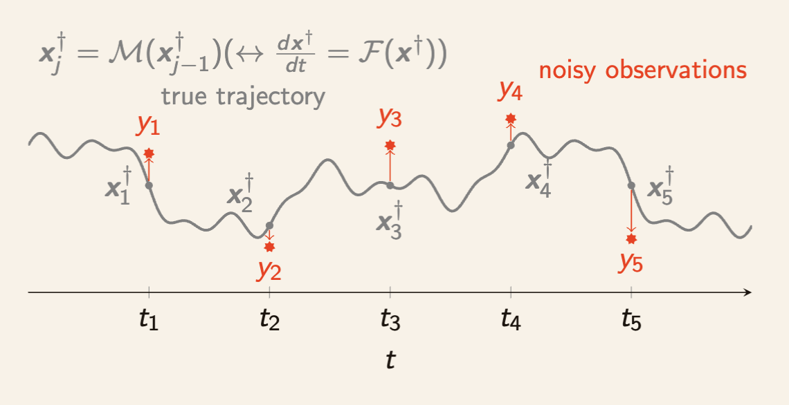
\frac{d x^\dagger}{dt} = \mathcal{F}(x^\dagger)
(\mathcal{F}: \mathbb{R}^{N_x} \rightarrow \mathbb{R}^{N_x})
y_j = H x^\dagger_j + \xi_j
(H: \mathbb{R}^{N_y \times N_x}, \xi_j \in \mathbb{R}^{N_y} \text{ noise})
x^\dagger_j = x^\dagger(jh)
Model dynamics
Observation
\mathbb{R}^{N_x}
\mathbb{R}^{N_y}
(h > 0 \text{ obs. interval})
Aim
x^\dagger_j
Unkown
Given
Y_j = \{y_i \mid i \le j\}
x_j
Construct
x^\dagger_j
estimate
Quality Assessment
\mathbb{E}\left[|x_j - x^\dagger_j|^2\right]
(\text{i.e. } \mathbb{P}^{x_j} \approx \mathbb{P}^{x^\dagger_j}({}\cdot{} | Y_j))
y_j
\mathbb{R}^{N_x}
\mathbb{R}^{N_y}
x^\dagger_{j-1}
x^\dagger_j
y_{j-1}
Given
Model
Obs.
Obs.
unknown
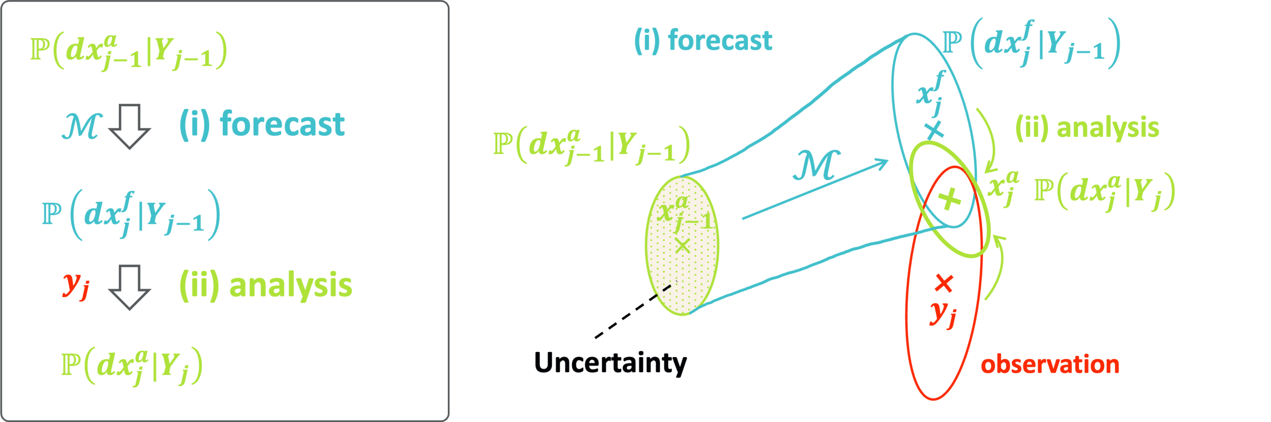
Sequential Data Assimilation
\mathbb{P}^{x_{j-1}}
\mathbb{P}^{\hat{x}_j}
\mathbb{P}^{x_j}
→ Next: approximate this numerically
Prediction
by Bayes' rule
\mathbb{P}^{x_j} = \mathbb{P}^{x^\dagger_j}({}\cdot{} \mid Y_j)
\Rightarrow
by model
Update
y_j
We can construct the exact distribution by 2 steps at each time step.
Data Assimilation Algorithms
Only focus on Approximate Gaussian Algorithms
Data Assimilation Algorithms
\mathbb{P}^{x_j} \approx \frac{1}{m} \sum_{k=1}^m \delta_{x_j^{(k)}}.
Kalman filter(KF) [Kalman 1960]
- All Gaussian distribution
- Update of mean and covariance.
Assume: linear F, Gaussian noises
Ensemble Kalman filter(EnKF)
Non-linear extension by Monte Carlo
- Update of ensemble
- Two major implementations:
- Perturbed Observation (PO): stochastic
- Ensemble Transform Kalman Filter (ETKF): deterministic
\mathbb{P}^{x_j} = \mathcal{N}(m_j, C_j).
x_j^{(1)},\dots,x_j^{(m)}.
Data Assimilation Algorithms
Kalman filter(KF)
Assume: linear F, Gaussian noises
Ensemble Kalman filter(EnKF)
Non-linear extension by Monte Carlo
Two implementations:
- PO: stochastic
- ETKF: deterministic
m_j, C_j
X_j
\widehat{m}_j, \widehat{C}_j
m_{j-1}, C_{j-1}
J(x) = \frac{1}{2} |y_j - Hx|_{R}^2 + \frac{1}{2} |x - \widehat{m}_j|_{\widehat{C}_j}^2
Regularized Least Squares
y_j
X_{j-1}
\widehat{X}_j
y_j
X_j = [x_j^{(k)}]_{k=1}^m, \widehat{X}_j = [\widehat{x}_j^{(k)}]_{k=1}^m.
Linear F
\text{nonlinear } \mathcal{F}
Bayes' rule
\Leftrightarrow
Regularized Least Squares
\widehat{m}_j, \widehat{C}_j
m_j, C_j
approx.
ensemble
\approx
\approx
predict
update
PO (stochastic EnKF)
\widehat{v}^{(k)}_j = \mathcal{M}(v^{(k)}_{j-1}), \quad k = 1, \dots, m.
y^{(k)}_j = y_j + \xi_j^{(k)}, \quad \xi_j^{(k)} \sim N(0, R), \quad k = 1, \dots, m.
(ii) \widehat{X}_j, y_j \rightarrow X_j: \text{Replicate observations,}\\
(i) X_{j-1} \rightarrow \widehat{X}_j: \text{ Evolve each member by model dynamics } \mathcal{M},
x_j^{(k)} = \widehat{x}_j^{(k)} + K_j(y_j^{(k)} - H \widehat{x}_j^{(k)}), \quad k = 1, \dots, m,
\text{Then, update each member,}
Stochastic!
(Burgers+1998) G. Burgers, P. J. van Leeuwen, and G. Evensen, Analysis Scheme in the Ensemble Kalman Filter,684, Mon. Weather Rev., 126 (1998), pp. 1719–1724.
\text{where } K_j = \widehat{C}_j H^\top (H \widehat{C}_j H^\top + R)^{-1}, \widehat{C}_j = \operatorname{Cov}(\widehat{X}_j),
ETKF (deterministic EnKF)
\widehat{v}^{(k)}_j = \mathcal{M}(v^{(k)}_{j-1}), \quad k = 1, \dots, m.
\text{with the transform matrix } T_j \in \mathbb{R}^{m \times m} \text{ s.t. }
(ii) \widehat{X}_j, y_j \rightarrow X_j: \text{Decompose } \widehat{X}_j =\overline{\widehat{x}}_j + d\widehat{X}_j.\\
(i) X_{j-1} \rightarrow \widehat{X}_j: \text{ Evolve each member by model dynamics } \mathcal{M},
\overline{x}_j = \overline{\widehat{x}}_j^{(k)} + K_j(y_j^{(k)} - H \overline{\widehat{x}}_j^{(k)}), \quad dX_j = d\widehat{X}_j T_j.
\text{Then, update separately,}
Deterministic!
(Bishop+2001)C. H. Bishop, B. J. Etherton, and S. J. Majumdar, Adaptive Sampling with the Ensemble Transform681
Kalman Filter. Part I: Theoretical Aspects, Mon. Weather Rev., 129 (2001), pp. 420–436.
\frac{1}{m-1} d\widehat{X}_j T_j (d\widehat{X}_j T_j)^* = (I - K_j H) \widehat{C}_j.
Inflation (numerical technique)
Issue: Underestimation of covariance through the DA cycle.
→ Poor state estimation.
→ (idea) inflating covariance before the update step.
Two basic methods of (covariance) inflation
\text{Additive } (\alpha \ge 0): \widehat{C}_j \rightarrow \widehat{C}_j + \alpha^2 I_{N_x} \text{ (only for PO)}.
\text{Multiplicative } (\alpha \ge 1): \widehat{C}_j \rightarrow \alpha^2\widehat{C}_j \text{ (PO)},
d\widehat{X}_j \rightarrow \alpha d\widehat{X}_j \text{ (ETKF)}.
\text{where } d\widehat{X}_j = [\widehat{x}^{(k)}_j - \overline{\widehat{x}}_j]_{k=1}^m, \overline{\widehat{x}}_j = \frac{1}{m} \sum_{k=1}^m \widehat{x}^{(k)}_j.
Literature review
-
Consistency (Mandel+2011, Kwiatkowski+2015)
-
Sampling errors (Al-Ghattas+2024)
-
Error analysis (full observation )
-
PO (Kelly+2014)
-
ETKF (T.+2024) → current
-
-
Error analysis (partial observation) → future
(Kelly+2014) D. T. B. Kelly, K. J. H. Law, and A. M. Stuart, Well-posedness and accuracy of the ensemble716
Kalman filter in discrete and continuous time, Nonlinearity, 27 (2014), pp. 2579–260.
(Al-Ghattas+2024) O. Al-Ghattas and D. Sanz-Alonso, Non-asymptotic analysis of ensemble Kalman updates: Effective669
dimension and localization, Information and Inference: A Journal of the IMA, 13 (2024).
(Kwiatkowski+2015) E. Kwiatkowski and J. Mandel, Convergence of the square root ensemble kalman filter in the large en-719
semble limit, Siam-Asa J. Uncertain. Quantif., 3 (2015), pp. 1–17.
(Mandel+2011) J. Mandel, L. Cobb, and J. D. Beezley, On the convergence of the ensemble Kalman filter, Appl.739 Math., 56 (2011), pp. 533–541.
H = I_{N_x}
How EnKF approximate KF?
How EnKF approximate
the true state?
Mathematical analysis of EnKF
Assumptions on model
(Reasonable)
Assumption on observation
(Strong)
Assumptions for analysis
N_y = N_x, H = I_{N_x}, \xi \sim \mathcal{N}(0, r^2 I_{N_x})
Assumption (obs-1)
full observation
Strong!
\exist \rho > 0 \text{ s.t. } \forall x_0 \in B(\rho), \forall t > 0, x(t ; x_0) \in B(\rho).
\exist \beta > 0 \text{ s.t. } \forall x \in B(\rho), \forall x' \in \mathbb{R}^{N_x},
\langle F(x) - F(x'), x - x' \rangle \le \beta | x - x'|^2.
\exist \beta > 0 \text{ s.t. } \forall x, x' \in B(\rho), |F(x) - F(x')| \le \beta | x - x'|.
Assumption (model-1)
Assumption (model-2)
Assumption (model-2')
\forall x_0 \in \R^{N_x}, \dot{x}(t) = F(x(t)) \text{ has an unique strong solution, and}
Reasonable
(B(\rho) = \{x \in \R^{N_x} \mid |x| \le \rho \})
Dissipative dynamical system
Dissipative dynamical systems
Lorenz' 63, 96 equations, widely used in geoscience,
\frac{dx^i}{dt} = (x^{i+1} - x^{i-2}) x^{i-1} - x^i + f \quad (i = 1, \dots, 40),
Example (Lorenz 96)
\bm{x} = (x^i)_{i=1}^{40} \in \mathbb{R}^{40}, f \in \R,
non-linear conserving
linear dissipating
forcing
Assumption (model-1, 2, 2')
hold
Example (Lorenz 63)
(incompressible 2D Navier-Stokes equations in infinite-dim. setting)
Error analysis of PO (prev.)
Theorem (Kelly+2014)
\text{Let us consider the PO method with additive inflation } \alpha > 0.
\limsup_{j \rightarrow \infty} e^{(k)}_j \le \frac{2\min\{m, N_x\}}{1-\theta}r^2.
\text{Then, } \exist \theta = \theta(\beta, h, r, \alpha) \in (0, 1), \text{ s.t. } k = 1, \dots, m,
\text{Let } e^{(k)}_j = \mathbb{E}\left[|x^{(k)}_j - x^\dagger_j|^2\right] \text{ for } k = 1, \dots, m.
\text{Let Assumptions (obs-1, model-1,2) hold and }\alpha \gg 1.
variance of observation noise
uniformly in time
Error analysis of ETKF (our)
\limsup_{j \rightarrow \infty} e_j \le \frac{N_x r^2}{1-\theta} + \left(\frac{1 - \Theta}{1 - \theta} - 1\right)D.
Theorem (T.+2024)
\text{Let } e_j = \mathbb{E}\left[|\overline{x}_j - x^\dagger_j|^2\right] \text{ where } \overline{x}_j = \frac{1}{m} \sum_{k=1}^m x^{(k)}_j.
\text{where } \Theta = \Theta(\beta, \rho, h, r, m, \alpha) , D = D(\beta, \rho).
\text{Let us consider the ETKF with multiplicative inflation } \alpha \ge 1.
\text{Then } \exist \theta = \theta(\beta, \rho, h, r, m, \alpha) < 1\text{ s.t.}
\text{Let Assumptions (obs-1, model-1,2') hold.}
\text{Suppose } m > N_x \text{ so that } \operatorname{rank}([x^{(k)}_0]_{k=1}^m) = N_x \text{ and } \alpha \gg 1,
Summary
\limsup_{j \rightarrow \infty} e^{(k)}_j \le \frac{2\min\{m, N_x\}}{1-\theta}r^2,
\limsup_{j \rightarrow \infty} e_j \le \frac{N_x r^2}{1-\theta} + \left(\frac{1 - \Theta}{1 - \theta} - 1\right)D.
\text{Suppose } m > N_x \text{ and } \alpha \gg 1,
\text{Suppose } \alpha \gg 1,
ETKF with multiplicative inflation (our)
PO with additive inflation (prev.)
= O(r^2)
r \rightarrow 0
accurate observation limit
= O(r^2)
O(r^4)
\text{for } k = 1, \dots, m.
Two approximate Gaussian filters (EnKF) are assessed in terms of the state estimation error.
due to
due to
Take home message
Data Assimilation is a seamless integration of
Data into Model.
Statistics/
Probability
Fluid Mechanics/
Other Dynamics
Numerical Analysis
There are still many problems in DA, and
we need to cooperate with a wide range of fields.
Optimization
Engineering
Machine Learning
Computing
Thank you for listening!
Please feel free to contact me.
Any Questions?
ensemble Kalman filter
(SIAM SC Kyoto)
Data Assimilation
Fluid mechanics
Future plans

Issue: partial observation
y = (x^1, x^2) + \xi
x = (x^1, x^2, x^3)
Partially observed
H
in Assumption (obs-1) is too strong for real-world applications.
H = I_{N_x}
In general, we can obtain partial information about the state.
Example
(full observation),
(H \text{ is a projection.})
Future plan
Error analysis with projection
Difficult to obtain the error bound with projection
→ need to use detailed properties of model dynamics.
Related studies (DA with noiseless observations)
H = \operatorname{diag}(1, 1, 0, 1, \dots, 0, 1, 1, 0, 1)
H = \operatorname{diag}(1, 0, 0)
we can reconstruct the true state in the time limit with
for Lorenz 63,
for Lorenz 96 (40-dim.).
If
R = O
(noiseless observations)
(Law+2015) K. J. H. Law, A. M. Stuart, and K. C. Zygalakis. Data Assimilation: A Mathematical Introduction. Springer, 2015.
(Law+2016) K. J. H. Law, D. Sanz-Alonso, A. Shukla, and A. M. Stuart. Filter accuracy for the Lorenz 96 model: Fixed versus adaptive observation operators. Phys. -Nonlinear Phenom., 325:1–13, 2016.
Mathematical Analysis of Ensemble Kalman Filter
By kotatakeda
Mathematical Analysis of Ensemble Kalman Filter
EASIAM 2024


