4 vs. 9 Classification Using Topological Data Analysis
Yifan Gu, Erin O'Neil, Kye Shi, & Mia Zender
(Math 285J)
Motivation:
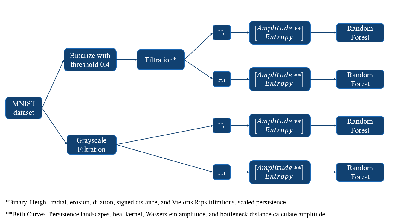
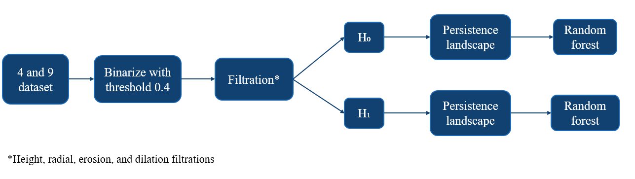
- We adapt the methodology presented in Garin & Tauzin's conference paper [1] that uses TDA to classify handwritten numbers based on the following pipeline:
[1] Adélie Garin, & Guillaume Tauzin. (2019). A Topological "Reading" Lesson: Classification of MNIST using TDA
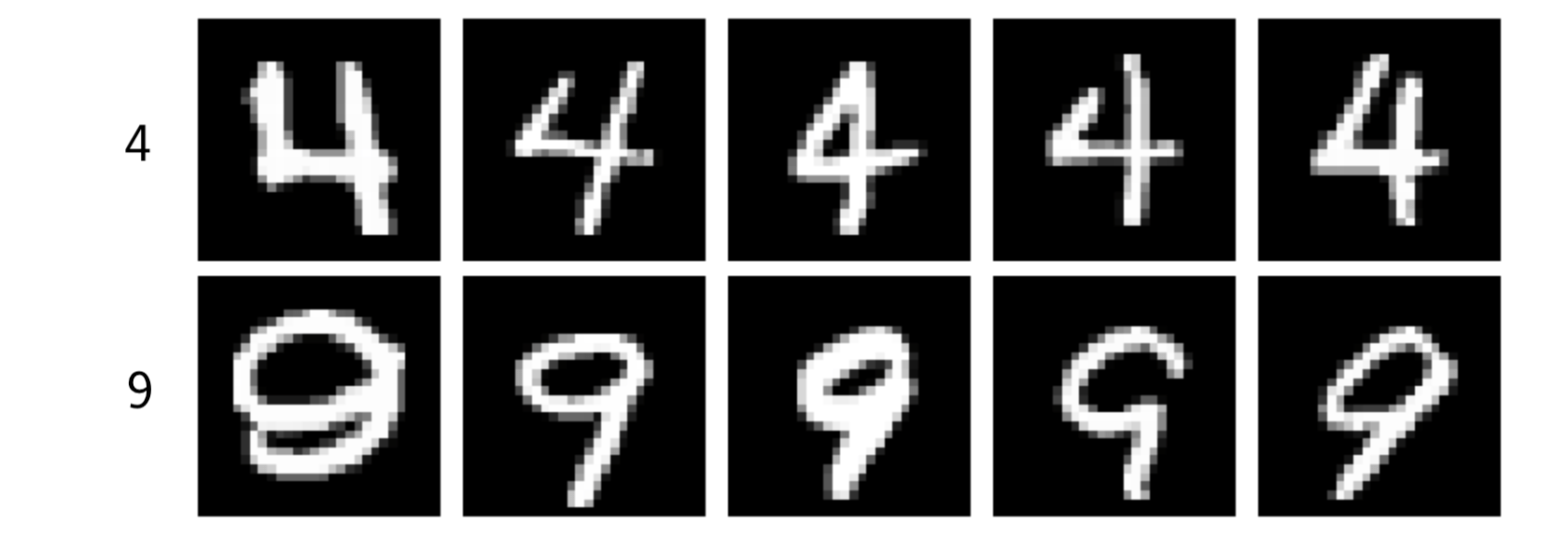
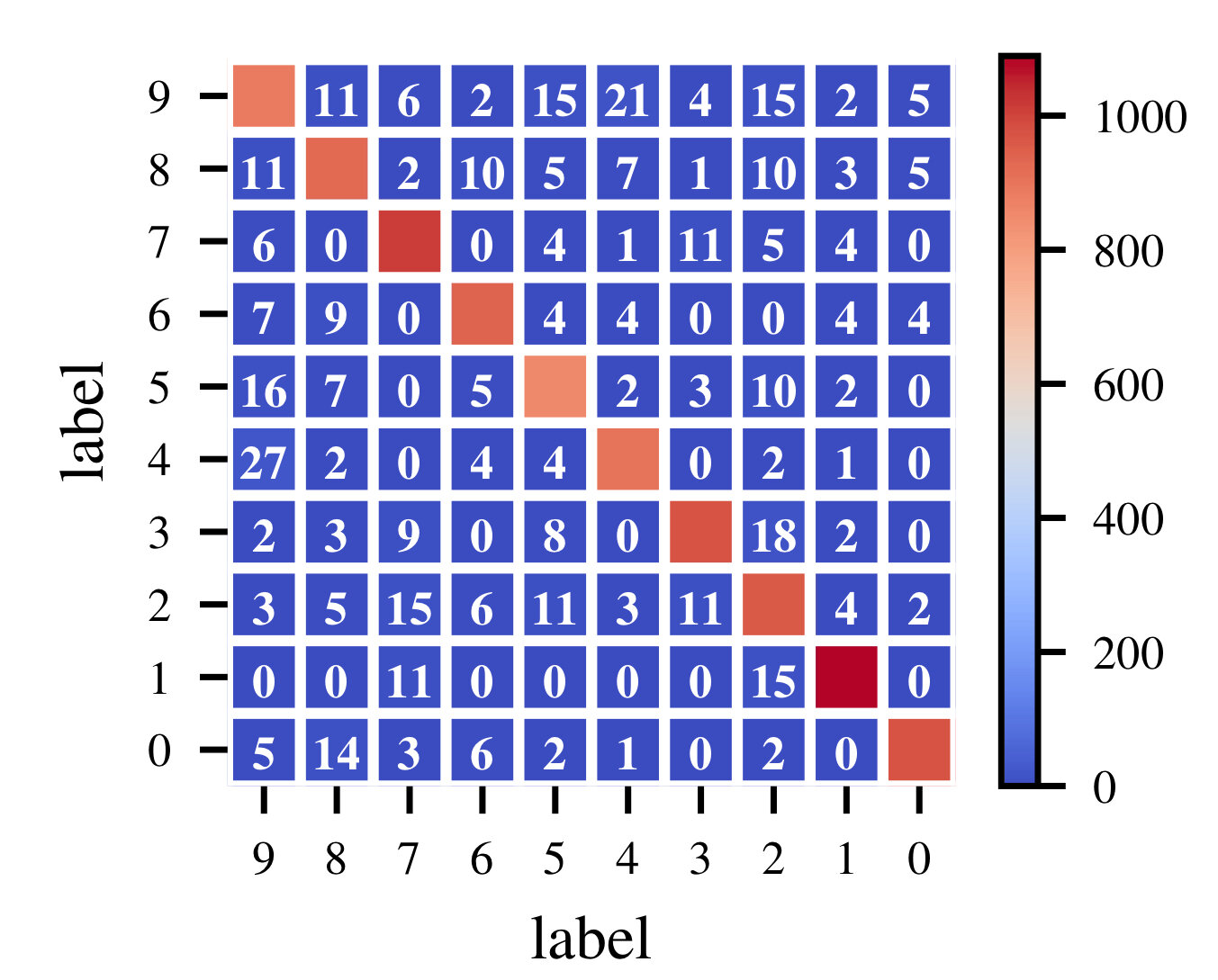
Data:
- We restrict our attention to the "4" and "9" numbers within the MNIST digits dataset due to their high classification error rate
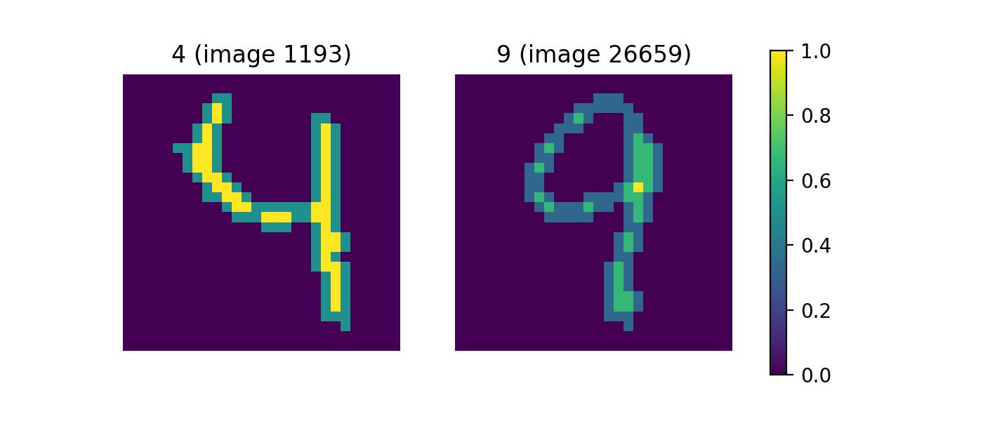
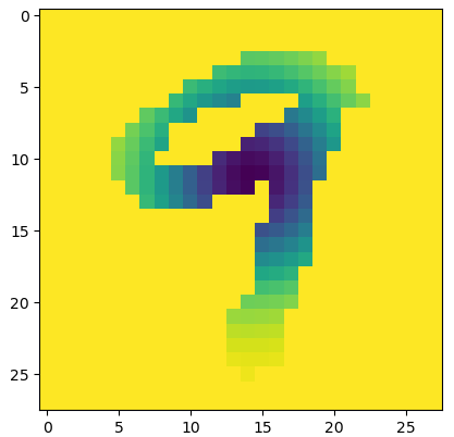
Cubical complex:
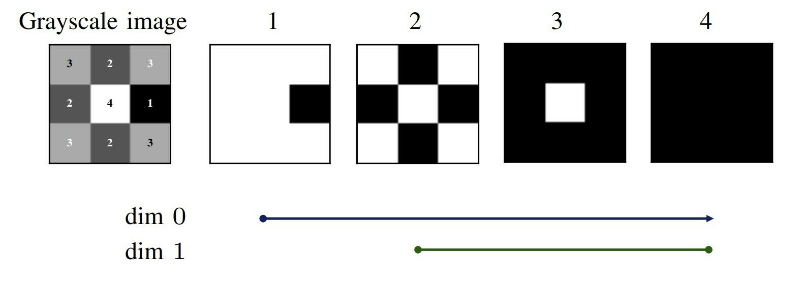
Note that there is one connected component in image 2 (diagonal pixels are considered to be a part of the same connected component).
Each pixel with intensity is represented by a vertex and cubes are created between vertices.
\mathcal{I}(v)
\sigma
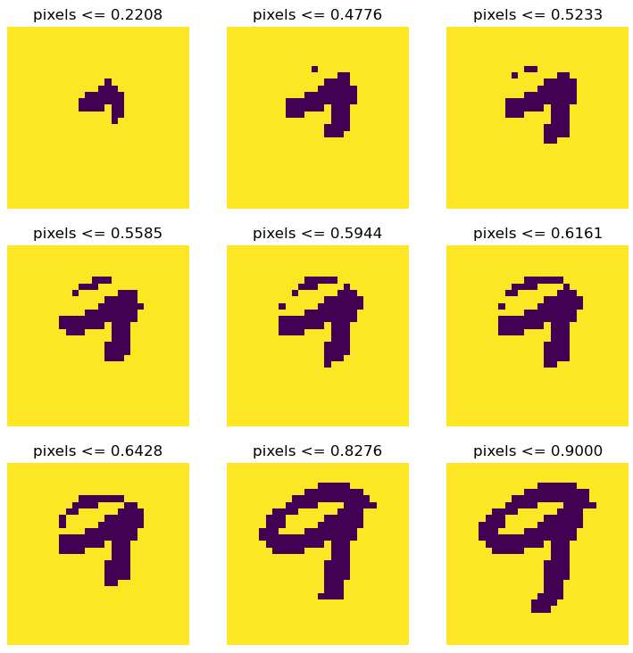
The image above has cubes indexed by their intensity and depicts a filtration of cubical complexes.
We explored the following questions:
- What filtration methods are useful for classifying the 4 vs. 9 digits?
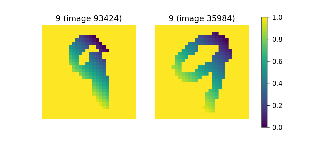
- Radial filtration (with choice of center):
Given center c, assign to pixel p the intensity value
where
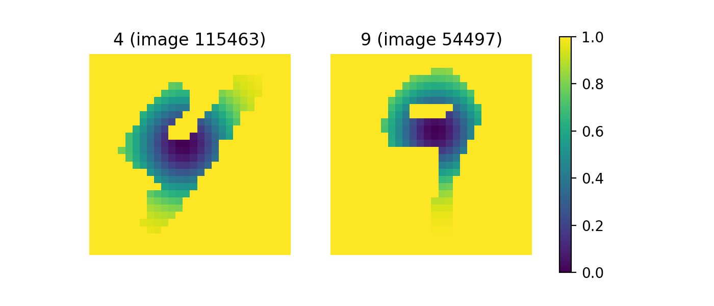
- Height filtration (with choice of direction):
Given direction v, assign to pixel p
where
\mathcal{R}(p):=\begin{cases}\|c-p\|_2 & p\in\mathcal{B} \\ \mathcal{R}_\infty & p\notin\mathcal{B}\end{cases}
\mathcal{R}_\infty:=\max_{p\in\mathcal{B}}\|c-p\|_2
\mathcal{H}(p):=\begin{cases}\langle p, v\rangle & p\in\mathcal{B}\\ \mathcal{H}_\infty & p\notin\mathcal{B}\end{cases}
\mathcal{H}_\infty:=\max_{p\in\mathcal{B}}\langle p,v\rangle
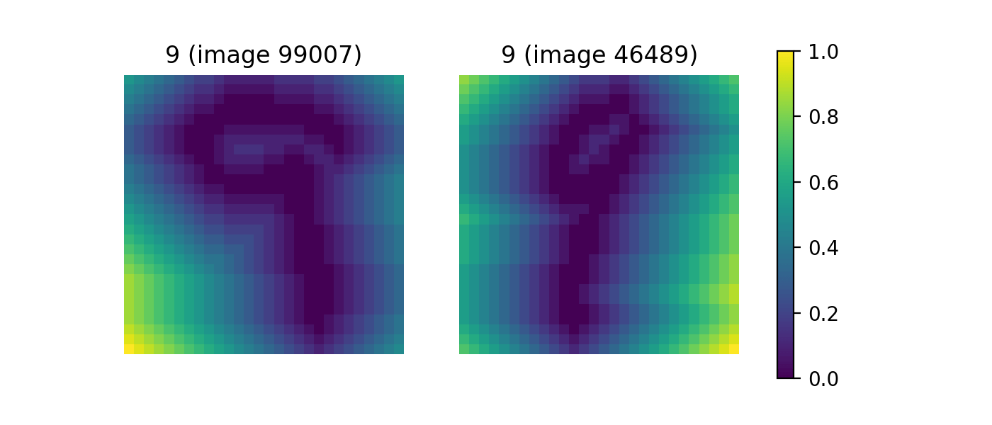
- Erosion
Erosion defines a new grayscale image, , at a vertex p is the distance from p to the closest vertex v that has binary value 0.
Note: If , then
- Dilation
i.e. applying erosion to the inverse image
Dilation defines a new grayscale image, , at a vertex p is the distance from p to the closest vertex v that has binary value 1.
Note: If , then
\mathcal{E}(p):=\min\{\|p-v\|_1:v\notin\mathcal{B}\}
\mathcal{D}(p):=\min\{\|p-v\|_1:v\in\mathcal{B}\}
p\notin\mathcal{B}
\mathcal{E}(p)=0
p\in\mathcal{B}
\mathcal{D}(p)=0
\mathcal{E}
\mathcal{D}
- Radial filtration from the center of mass
Example of filtration:
Gif of example filtration! (radial?)
And corresponding persistent diagram?
- This is an example of a binarized image
Questions continued...
- Which approaches of generating features lead to the best predictive power?
- How tolerant is our methodology to noise?
- Are there practical uses of this TDA-ML pipeline (i.e. is it faster/better than other algorithms)?
Predictors used by Garin & Tauzin
| Betti Curves | Heat Kernel | Persistence Landscapes |
|---|---|---|
|
Describes the number of barcodes an x on the vertical axis is contained in |
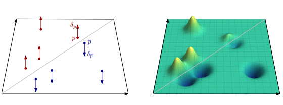
Gaussians with certain standard deviations are placed over each birth-death pair in the persistence diagram. A negative Gaussian with the same standard deviation is placed across the diagonal in the persistence diagram as well. The kernel maps to . The paper mentions in their "filtration units" |
More on a later slide. |
| Wasserstein Amplitude | Bottleneck Amplitude |
|---|---|
|
|
Amplitude
A=\frac{\sqrt{2}}{2}\sum_{i=1}^n(d_i-b_i)
A=\frac{\sqrt{2}}{2}\bigg(\sum_{i=1}^n(d_i-b_i)^2\bigg)^{1/2}
A=\frac{\sqrt{2}}{2}\max_{1\leq i\leq n}(d_i-b_i)
Note: This is all for a persistence diagram D with birth death pairs .
\{(b_i,d_i)\}_{i=1}^n
J. Reininghaus, S. Huber, U. Bauer, and R. Kwitt, “A stable multi-scale kernel for topological machine learning,” in 2015 IEEE Conference on Computer Vision and Pattern Recognition (CVPR), June 2015, pp. 4741– 4748.
\mathbb{R}^2
\sigma=10,15
B_k(x)=\#\{(b_j,d_j):x\in(b_j,d_j)\}
k\in\{0,1\}
Predictors used by Garin & Tauzin
Persistent Entropy:
PE=-\sum_{i=1}^n\frac{l_i}{L}\log \bigg(\frac{l_i}{L}\bigg)
l_i=d_i-b_i
L=\sum_{i=1}^nl_i
where and
\begin{bmatrix} A\\PE\end{bmatrix}
Note: This is all for a persistence diagram D with birth death pairs .
\{(b_i,d_i)\}_{i=1}^n
is the input to the random forest
A is one of the amplitudes from the previous slide and PE is the persistent entropy
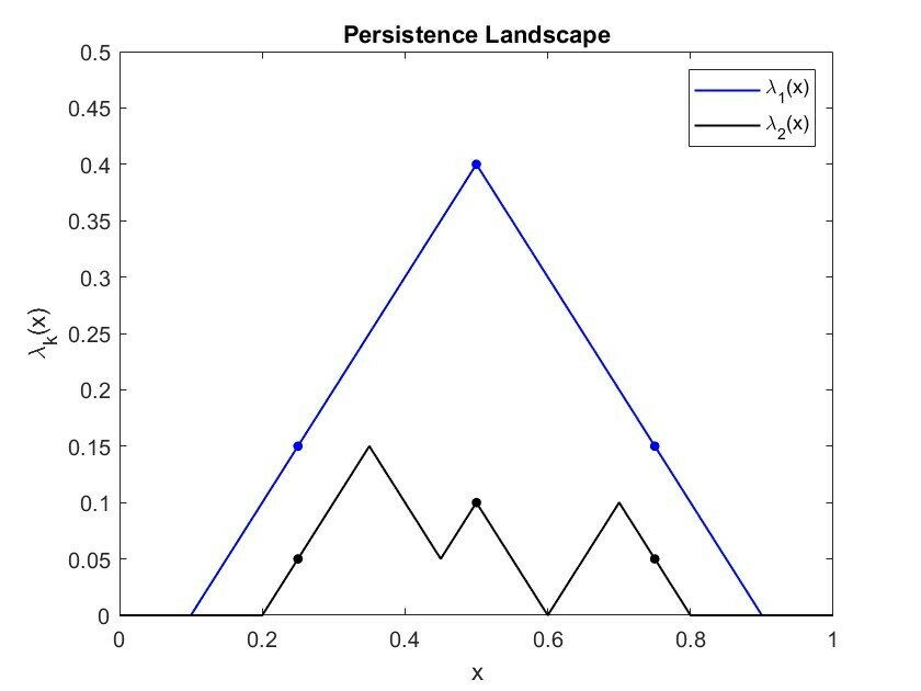
Persistence Landscapes:
f_{(b_i,d_i)}(x)=\begin{cases}
0, x\notin (b_i,d_i)\\
x-b_i, x\in\big(b_i,\frac{b_i+d_i}{2}\big)\\
-x+d_i, x\in\big(\frac{b_i+d_i}{2},d_i\big)\\
\end{cases}
Given n birth death pairs in a persistence diagram, define:
for each birth death pair,
(b_i,d_i).
Then, define the first persistence landscape:
\lambda_1(x)=\max_{1\leq i\leq n}\{f_{(b_i,d_i)}(x)\}
Also define the second persistence landscape:
\lambda_2(x)=\max_{1\leq i\leq n}\{f_{(b_i,d_i)}(x):f_{(b_i,d_i)}(x)\neq\lambda_1(x)\}
Garin &Tauzin found and for 100 sample
\lambda_1(x_j)
\lambda_2(x_j)
x_j\in[0,1]
and calculated amplitudes
\|\lambda_1(x)\|_1\text{, } \|\lambda_1(x)\|_2\ \text{, } \bigg\|\begin{bmatrix}
\lambda_1(x)\\ \lambda_2(x)
\end{bmatrix}\bigg\|_1\text{, }
\bigg\|\begin{bmatrix}\lambda_1(x)\\ \lambda_2(x)\end{bmatrix}\bigg\|_2
where and
\lambda_1(x)=[\lambda_1(x_1),\dots,\lambda_1(x_{100})]^T
\lambda_2(x)=[\lambda_2(x_1),\dots,\lambda_2(x_{100})]^T
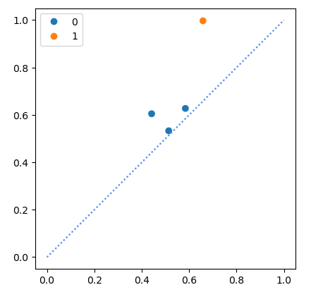
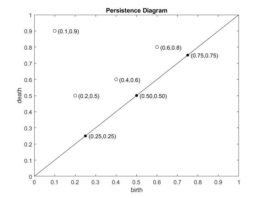
Persistence Landscapes Example :
| 0.25 | 0.15 | 0.05 | 0 | 0 | 0.15 | 0.05 |
| 0.5 | 0.4 | 0 | 0.1 | 0 | 0.4 | 0.1 |
| 0.75 | 0.15 | 0 | 0 | 0.05 | 0.15 | 0.05 |
x
f_{(0.1,0.9)}(x)
f_{(0.2,0.5)}(x)
f_{(0.4,0.6)}(x)
f_{(0.6,0.8)}(x)
\lambda_1(x)
\lambda_2(x)
Overview of Our Pipeline:
We create an ensemble TDA-ML algorithm inspired by Garin & Tauzin that combines the predictions of many filtration methods to yield a single prediction:
We keep the following consistent with Garin & Tauzin: image binarization using a threshold value of 0.4, choice of simplicial complex (cubical), choice of machine learning algorithm (random forest). We also use a subset of their filtration methods. We elected not to scale the images using the process by Garin and Tauzin due to errors in the code.
Results: (i) Effect of number of features
| Number of features | Prediction accuracy |
|---|---|
| 784 | 0.9903 |
| 576 | 0.9858 |
| 384 | 0.9867 |
| 192 | 0.9836 |
- More features might very slightly improve performance, but not meaningfully outside of random fluctuations
- However, even ~1/4 of the original feature size is enough to produce a very close accuracy, showing that the condensed features do capture the data well
Results: (ii) Comparison between H0 and H1
| Number of features | Homology group | Prediction accuracy |
|---|---|---|
| 96 | H0 | 0.8824 |
| 96 | H1 | 0.9819 |
| 192 | H0 | 0.9129 |
| 192 | H1 | 0.9828 |
| 288 | H0 | 0.9133 |
| 288 | H1 | 0.9836 |
H0 features perform significantly worse than H1 features, so we do not lose much without using them
Results: (iii) Comparison among filtrations
| Filtration | Prediction accuracy |
|---|---|
| Height | 0.9584 |
| Radial | 0.9447 |
| Dilation | 0.8969 |
| Erosion | 0.6329 |
Dilation performs much better than erosion, so we should drop erosion and focus on enhancing height and radial filtrations
Results: (iv) Comparison among metrics
| Metric | Prediction accuracy |
|---|---|
| Persistence entropy | 0.9584 |
| Wasserstein distance | 0.9841 |
| Bottleneck distance | 0.9398 |
| Persistence landscape | 0.9788 |
We should try to enhance Wasserstein distance and persistence landscape
Results: (v) Mini summary
- We finally focus on two ways of feature generation:
- 11 filtrations x 8 metrics = 88 features in total, ~10% of original dimension; prediction accuracy = 0.9805
- 18 filtrations x 14 metrics = 252 features, ~1/3 of the original; prediction accuracy = 0.9867
- Condensed topological information, even just that of H1, is enough to capture the original data well, an idea of conceptual importance
- Both accuracies < 0.99; might consider other metrics to further improve (e.g. persistence silhouette function, Euler characteristic curve, ...)
- Practically, generating features takes O(10) minutes, whereas traditional random forest is real-time
We now look at how robust TDA-enhanced ML can be against noise.
Noise Experiment:
Noise was generated by sampling a gaussian distribution with mean 0 and standard deviation equal to noise level. We consider 3 levels of noise.
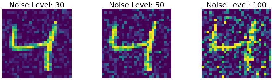
Noise Experiment Results:
| Noise level | Random Forest | TDA approach |
|---|---|---|
| 30 | 0.989 | 0.975 |
| 50 | 0.983 | 0.879 |
| 100 | 0.966 | 0.838 |
The TDA approach performed poorer than the Random Forest classifier. In addition, the TDA approach was more computationally expensive. Therefore, there does not seem to be any benefits to the TDA approach when handling noisy data.
Hypothesis: TDA approach has a convoluted persistence diagram with noise that becomes hard to extract features from/learn from
Conclusion:
Given more time, we would further explore...
- Our TDA approach was not robust to noise
- The traditional random forest algorithm seems to be a more optimal choice for classifying the 4 versus 9 dataset based on our observations so far
-Can features be extracted by sampling persistence landscapes themselves (as opposed to taking norms)?
- Are there any applications where the TDA approach outperforms random forest (e.g. under rotations?)
deck
By kyeshi98