Parameterized Quantum Circuits
Min-Hsiu Hsieh
University of Technology Sydney, Australia
and Its Applications in Machine Learning
Machine Learning Tasks


PQC Can Achieve


"In computational complexity-theoretic terms, this generally means providing a superpolynomial speedup over the best possible classical algorithm."
Quantum supremacy

QML applications are natural candidates for NISQ devices.
Part I
Parameterized Quantum
Circuits


and many more!

PQC
q(X)
\theta
Classical Optimization
Classical Optimization
\theta = \arg \min_{\bm{\theta}} \mathcal{L}(q(X),p(X))
Given an loss function \(\mathcal{L}\), PQC output \(q(X)\), a target distribution \(p(X)\),
Part II
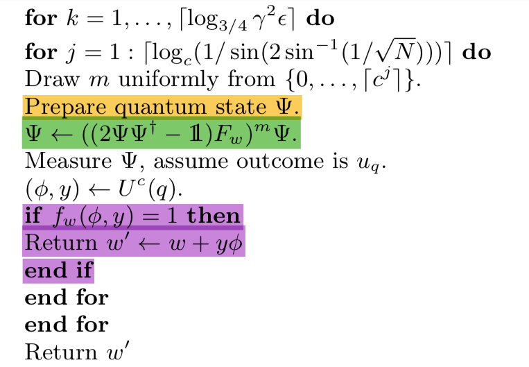
PQC as Quantum Perceptron


and more!

Quantum Perceptron
Grover Search
P_\omega= |\omega\rangle\langle \omega|
P_s= |+\rangle\langle +|^{\otimes n}
U_s= 2|+\rangle\langle +|^{\otimes n} - I
U_\omega= 2|\omega\rangle\langle \omega| - I
How to identify
from
Grover Search

Variational Grover Search
\min_{\phi} \langle \phi |P_{\omega^\perp} | \phi\rangle
Learn \(|\phi\rangle\) using trainable quantum circuits.
Morales, Tlyachev, and Biamonte. Variationally Learning Grover’s Quantum Search Algorithm. arXiv:1805.09337
U(\alpha) = e^{i\alpha P_\omega}
V(\beta) = e^{i\beta P_s}
Variational Grover Search

Variational Quantum Perceptron

Variational Quantum Perceptron
\mathcal{D} = \{\bm{x}_i \in \mathbb{R}^M, y_i\in\{\pm 1\}\}_{i=1}^N
|\Phi^{(k)}\rangle_{F,I}= U_{data}(\mathcal{D})
=\frac{1}{\sqrt{N}}\left(\sum_{i=0,i\neq k}^{N-1}|\psi_i^{(0)}\rangle_{F}|i\rangle_I -|\psi_k^{(1)}\rangle_{F}|k\rangle_I\right).
Variational Quantum Perceptron
U_{c1}|\Phi^k\rangle_{F,I}=|\varphi\rangle_F\otimes\left(\cos3\theta|B\rangle_I+\sin3\theta|k\rangle_I\right)
U_{L_1}|{\Phi^k}\rangle_{F,I}= \cos\theta(\textcolor{red}{\alpha_B}|\psi_B^{(0)}\rangle_F+ \textcolor{green}{\beta_k}|\psi_k^{(1)}\rangle_F)|{B}\rangle_I + \sin\theta(-\textcolor{red}{\alpha_B}|\psi_B^{(0)}\rangle_F+ \textcolor{green}{\beta_k}|\psi_k^{(1)}\rangle_F)|{k}\rangle_I
VQP Performance

N=16, M=4
Performance
N=16, M=4

Quantum Ensemble Learning
Combine weak VQP \(\{V_t\}\) into strong classifier \(\rm{sign}(\sum_t |y_t - C_T|)\).
Required significant smaller size of training sets
QEL Complexity
Query Complexity \(O(\textcolor{red}{T}\text{poly}(\log M\textcolor{green}{\sqrt{\log N}}))\).
Runtime \(O(\text{poly}(\log M \log( M\sqrt{\log N}))\sqrt{\log N})\).
If \(|\mathcal{D}_t|\approx \log {N} \)
QEL Performance
\( \mathcal{D}=\{\bm{x}_i,y_i\}_{i=1}^{10000} \)
\( \mathcal{D}_i=\{\bm{x}_k,y_k\}_{k=1}^{8} \)

Gate Count
\( \mathcal{D}=\{\bm{x}_i,y_i\}_{i=1}^{10000} \)
\( \mathcal{D}_i=\{\bm{x}_k,y_k\}_{k=1}^{8} \)
Encoding requires 29 single and two qubits gates.
QEL requires 48 parameterized single qubit gates, 8 CNOT gates, 12 NOT gates, 20 Hadamard gates, and 10 Toffoli gates.
Total of 248 single and two-qubit gates.
Part III
The Expressive Power of Parameterized Quantum Circuits
What is the generative power of parametrized quantum circuits?

MPQC
- arXiv:1801.07686, arXiv:1804.04168
TPQC

arXiv:1803.11537
Boltzmann Machine

Boltzmann Machine

MPQC\(>\)DBM\(>\)TPQC\(>\)RBM
Expressive Power:

IQP circuits
MPQC\(>\)DBM

IQP Circuit Can be simulated by MPQCs with the following arrangement.


DBM\(>\)TPQC

TPQC\(>\)RBM
TPQC can generate entangled state with volume law (Bond Dimension \(O(D^N)\)).
RBM Cannot!
-
Gao and Duan, Nature Communications 8, 662 (2017).
-
Chen et. al., Physical Review B 97, 085104 (2018).
MPQC with Post-Selection

MPQC with post-selection can simulate General Tensor Networks.


Part VI
Quantum Divide-and-Conquer GAN

Seth Lloyd and Christian Weedbrook. "Quantum generative adversarial learning". Phys. Rev. Lett. 121, 040502 (2018)

Generative Adversarial Network

Thank you for your attention!
Quantum Machine Learning
By Lawrence Min-Hsiu Hsieh
Quantum Machine Learning
QI school at Kyoto University, 18-20 of March 2019
- 724


