CS6015: Linear Algebra and Random Processes
Lecture 21: Principal Component Analysis (the math)
Learning Objectives
What is PCA?
What are some applications of PCA?
Recap of Wishlist
Represent the data using fewer dimensions such that
the data has high variance along these dimensions
the covariance between any two dimensions is low
the basis vectors are orthonormal
\mathbf{u_1} = \begin{bmatrix}1\\0\end{bmatrix}
\begin{bmatrix}x_{11}\\x_{12}\end{bmatrix}

\mathbf{u_2} = \begin{bmatrix}0\\1\end{bmatrix}
\mathbf{v_2}
\mathbf{v_1}
We will keep the wishlist aside for now and just build some background first (mostly recap)
Projecting onto one dimension
\begin{bmatrix}
x_{11}&x_{12}&x_{13}&x_{14}& \dots &x_{1n} \\
x_{21}&x_{22}&x_{23}&x_{24}& \dots &x_{2n} \\
x_{31}&x_{32}&x_{33}&x_{34}& \dots &x_{3n} \\
\dots &\dots &\dots &\dots &\dots &\dots \\
\dots &\dots &\dots &\dots &\dots &\dots \\
x_{m1}&x_{m2}&x_{m3}&x_{m4}& \dots &x_{mn} \\
\end{bmatrix}
\mathbf{X_1}^\top
\mathbf{X_2}^\top
\mathbf{X_3}^\top
\mathbf{X_m}^\top
\mathbf{X_4}^\top
\mathbf{X}
\mathbf{x_1} = x_{11}\mathbf{u_1} + x_{12}\mathbf{u_2} + \dots + x_{1n}\mathbf{u_n}
Standard Basis Vectors
(unit norms)
\begin{bmatrix}
\uparrow\\
\\
v1
\\
\\
\downarrow
\end{bmatrix}
New Basis Vector
(unit norm)
\mathbf{x_1} = \hat{x_{11}}\mathbf{v1}
\hat{x_{11}} = \frac{\mathbf{x_1}^\top \mathbf{v1}}{\mathbf{v1}^\top \mathbf{v1}} = \mathbf{x_1}^\top \mathbf{v1}
\mathbf{x_2} = \hat{x_{21}}\mathbf{v1}
\hat{x_{21}} = \frac{\mathbf{x_2}^\top \mathbf{v1}}{\mathbf{v1}^\top \mathbf{v1}} = \mathbf{x_2}^\top \mathbf{v1}
\mathbf{u2} = \begin{bmatrix} 0\\1 \end{bmatrix}
\mathbf{u1} = \begin{bmatrix} 1\\0 \end{bmatrix}
\begin {bmatrix}
x_{11}\\
x_{12}
\end {bmatrix}

Projecting onto two dimensions
\begin{bmatrix}
x_{11}&x_{12}&x_{13}&x_{14}& \dots &x_{1n} \\
x_{21}&x_{22}&x_{23}&x_{24}& \dots &x_{2n} \\
x_{31}&x_{32}&x_{33}&x_{34}& \dots &x_{3n} \\
\dots &\dots &\dots &\dots &\dots &\dots \\
\dots &\dots &\dots &\dots &\dots &\dots \\
x_{m1}&x_{m2}&x_{m3}&x_{m4}& \dots &x_{mn} \\
\end{bmatrix}
\mathbf{X_1}^\top
\mathbf{X_2}^\top
\mathbf{X_3}^\top
\mathbf{X_m}^\top
\mathbf{X_4}^\top
\mathbf{X}
\begin{bmatrix}
\uparrow & \uparrow
\\
\\
\mathbf{\scriptsize v_1} & \mathbf{\scriptsize v_2}
\\
\\
\downarrow & \downarrow
\end{bmatrix}
new basis vectors
(unit norm)
\mathbf{x_1} = \hat{x_{11}}\mathbf{v_1}+\hat{x_{12}}\mathbf{v_2}
\hat{x_{11}} = \mathbf{x_1}^\top \mathbf{v_1}
\mathbf{x_2} = \hat{x_{21}}\mathbf{v_1}+\hat{x_{22}}\mathbf{v_2}
\hat{x_{21}} = \mathbf{x_2}^\top \mathbf{v_1}
\mathbf{u_2} = \begin{bmatrix} 0\\1 \end{bmatrix}
\mathbf{u_1} = \begin{bmatrix} 1\\0 \end{bmatrix}
\begin {bmatrix}
x_{11}\\
x_{12}
\end {bmatrix}
\mathbf{\hat{\textit{X}}} =
\begin{bmatrix}
\hat{x_{11}}&\hat{x_{12}}\\
\hat{x_{21}}&\hat{x_{22}}\\
\hat{x_{31}}&\hat{x_{32}}\\
\dots &\dots\\
\dots &\dots\\
\hat{x_{m1}}&\hat{x_{m2}}\\
\end{bmatrix}
\mathbf{=}
\begin{bmatrix}
\mathbf{x_{1}}^\top \mathbf{v_{1}}&\mathbf{x_{1}}^\top \mathbf{v_{2}} \\
\mathbf{x_{2}}^\top \mathbf{v_{1}}&\mathbf{x_{2}}^\top \mathbf{v_{2}} \\
\mathbf{x_{3}}^\top \mathbf{v_{1}}&\mathbf{x_{3}}^\top \mathbf{v_{2}} \\
\dots &\dots \\
\dots &\dots \\
\mathbf{x_{m}}^\top \mathbf{v_{1}}&\mathbf{x_{m}}^\top \mathbf{v_{2}} \\
\end{bmatrix}
\mathbf{= \textit{XV}}
\hat{x_{12}} = \mathbf{x_1}^\top \mathbf{v_2}
\hat{x_{21}} = \mathbf{x_2}^\top \mathbf{v_2}
\mathbf{v_1}
\mathbf{\textit{V}}
\mathbf{v_2}
Projecting onto k dimension
\begin{bmatrix}
\hat{x_{11}}&\hat{x_{12}}& \dots &\hat{x_{1k}} \\
\hat{x_{21}}&\hat{x_{22}}& \dots &\hat{x_{2k}} \\
\hat{x_{31}}&\hat{x_{32}}& \dots &\hat{x_{3k}} \\
\dots &\dots &\dots &\dots \\
\dots &\dots &\dots &\dots \\
\hat{x_{m1}}&\hat{x_{m2}}& \dots &\hat{x_{mk}} \\
\end{bmatrix}
\mathbf{X_1}^\top
\mathbf{X_2}^\top
\mathbf{X_3}^\top
\mathbf{X_m}^\top
\mathbf{X_4}^\top
\mathbf{\textit{X}}
\begin{bmatrix}
\uparrow & \uparrow & \cdots & \uparrow
\\
\\
\mathbf{\scriptsize v1} & \mathbf{\scriptsize v2} & \cdots & \mathbf{\scriptsize vk}
\\
\\
\downarrow & \downarrow & \cdots & \downarrow
\end{bmatrix}
     New Basis Vectors
       (unit norm)
\begin{bmatrix}
x_{11}&x_{12}&x_{13}&x_{14}& \dots &x_{1n} \\
x_{21}&x_{22}&x_{23}&x_{24}& \dots &x_{2n} \\
x_{31}&x_{32}&x_{33}&x_{34}& \dots &x_{3n} \\
\dots &\dots &\dots &\dots &\dots &\dots \\
\dots &\dots &\dots &\dots &\dots &\dots \\
x_{m1}&x_{m2}&x_{m3}&x_{m4}& \dots &x_{mn} \\
\end{bmatrix}
\mathbf{\hat{\textit{X}}} =
\mathbf{\textit{V}}
\begin{bmatrix}
\mathbf{x_{1}}^\top \mathbf{v_{1}}&\mathbf{x_{1}}^\top \mathbf{v_{2}}&\dots&\mathbf{x_{1}}^\top \mathbf{v_{k}} \\
\mathbf{x_{2}}^\top \mathbf{v_{1}}&\mathbf{x_{2}}^\top \mathbf{v_{2}}&\dots&\mathbf{x_{2}}^\top \mathbf{v_{k}}\\
\mathbf{x_{3}}^\top \mathbf{v_{1}}&\mathbf{x_{3}}^\top \mathbf{v_{2}}&\dots&\mathbf{x_{3}}^\top \mathbf{v_{k}} \\
\dots &\dots &\dots &\dots \\
\dots &\dots &\dots &\dots \\
\mathbf{x_{m}}^\top \mathbf{v_{1}}&\mathbf{x_{m}}^\top \mathbf{v_{2}}&\dots&\mathbf{x_{m}}^\top \mathbf{v_{k}} \\
\end{bmatrix}
\mathbf{= \textit{XV}}
\mathbf{=}
We want to find a V such that
columns of V are ortho-normal
columns of \(\mathbf{\hat{\textit{X}}}\) have high variance
What is the new covariance matrix?
\hat{X} = XV
\hat{\Sigma} = \frac{1}{m}\hat{X}^T\hat{X}
\hat{\Sigma} = \frac{1}{m}(XV)^T(XV)
\hat{\Sigma} = V^T(\frac{1}{m}X^TX)V
What do we want?
\hat{\Sigma}_{ij} = Cov(i,j)
\text{ if } i \neq j
low covariance
= 0
= \sigma^2_i
\text{ if } i = j
\neq 0
high variance
We want \( \hat{\Sigma}\) to be diagonal
We are looking for orthogonal vectors which will diagonalise \( \frac{1}{m}X^TX\) :-)
These would be eigenvectors of \( X^TX\)
(Note that the eigenvectors of cA are the same as the eigenvectors of A)
The eigenbasis of \(X^TX\)
\hat{\Sigma} = V^T(\frac{1}{m}X^TX)V = D
We have found a \( V \) such that
columns of \( V\) are orthonormal
eigenvectors of a symmetric matrix
columns of \( \hat{X}\) have zero covariance
diagonal
The right basis to use is the eigenbasis of \(X^TX\)
What about the variance of the columns of \( \hat{X}\) ?
?
\checkmark
\checkmark
What is the variance of the cols of \(\hat{X}\) ?
The i-th column of \(\hat{X}\) is
The variance for the i-th column is
The i-th column of \(\hat{X}\) is
\(\sigma_{i}^{2}\) = \(\frac{1}{m}\hat{X}_i^{T}\hat{X}_i\)
\mathbf{\textit{X}}
\begin{bmatrix}
\uparrow & \uparrow & \cdots & \uparrow
\\
\\
\mathbf{\scriptsize v1} & \mathbf{\scriptsize v2} & \cdots & \mathbf{\scriptsize vk}
\\
\\
\downarrow & \downarrow & \cdots & \downarrow
\end{bmatrix}
\begin{bmatrix}
x_{11}&x_{12}&x_{13}&x_{14}& \dots &x_{1n} \\
x_{21}&x_{22}&x_{23}&x_{24}& \dots &x_{2n} \\
x_{31}&x_{32}&x_{33}&x_{34}& \dots &x_{3n} \\
\dots &\dots &\dots &\dots &\dots &\dots \\
\dots &\dots &\dots &\dots &\dots &\dots \\
x_{m1}&x_{m2}&x_{m3}&x_{m4}& \dots &x_{mn} \\
\end{bmatrix}
\mathbf{\textit{V}}
\begin{bmatrix}
\mathbf{x_{1}}^\top \mathbf{v_{1}}&\mathbf{x_{1}}^\top \mathbf{v_{2}}&\dots&\mathbf{x_{1}}^\top \mathbf{v_{k}} \\
\mathbf{x_{2}}^\top \mathbf{v_{1}}&\mathbf{x_{2}}^\top \mathbf{v_{2}}&\dots&\mathbf{x_{2}}^\top \mathbf{v_{k}}\\
\mathbf{x_{3}}^\top \mathbf{v_{1}}&\mathbf{x_{3}}^\top \mathbf{v_{2}}&\dots&\mathbf{x_{3}}^\top \mathbf{v_{k}} \\
\dots &\dots &\dots &\dots \\
\dots &\dots &\dots &\dots \\
\mathbf{x_{m}}^\top \mathbf{v_{1}}&\mathbf{x_{m}}^\top \mathbf{v_{2}}&\dots&\mathbf{x_{m}}^\top \mathbf{v_{k}} \\
\end{bmatrix}
The variance for the i-th column is
\(\hat{X}_i \) = \( Xv_{i} \)
\mathbf{\hat{X} =}
\mathbf{\hat{X}_{1} }
\mathbf{\hat{X}_{2} }
\mathbf{\hat{X}_{n} }
The i-th column of \(\hat{X}\) is
The variance for the i-th column is
\(\hat{X}_i \) = \( Xv_{i} \)
\(\sigma_{i}^{2}\) = \(\frac{1}{m}\hat{X}_i^{T}\hat{X}_i\)
= \(\frac{1}{m}{(Xv_i)}^{T}Xv_i\)
= \(\frac{1}{m}{v_i}^T{X}^{T}Xv_i\)
= \(\frac{1}{m}{v_i}^T\lambda _iv_i\)
= \(\frac{1}{m}{(Xv_i)}^{T}Xv_i\)
= \(\frac{1}{m}{v_i}^T{X}^{T}Xv_i\)
= \(\frac{1}{m}{v_i}^T\lambda _iv_i\)
= \(\frac{1}{m}\lambda _i\)
= \(\frac{1}{m}\lambda _i\)
\((\because {v_i}^Tv_i = 1)\)
The full story
(How would you do this in practice?)
Compute the n eigen vectors of X TX
Sort them according to the corresponding eigenvalues
Retain only those eigenvectors corresponding to the top-k eigenvalues
Project the data onto these k eigenvectors
We know that n such vectors will exist since it is a symmetric matrix
These are called the principal components
Heuristics: k=50,100 or choose k such that λk/λmax > t
Reconstruction Error
\mathbf{x} =
\begin{bmatrix}x_{11}\\x_{12}\end{bmatrix} =
\begin{bmatrix}3.3\\3\end{bmatrix}
Suppose
\mathbf{x} = {3.3u_{1} + 3u_{2}}
Let
\mathbf{v_{1}} = \begin{bmatrix}1\\1\end{bmatrix}
\mathbf{v_{2}} = \begin{bmatrix}-1\\1\end{bmatrix}
\mathbf{v_{1}} = \begin{bmatrix}\frac{\mathbf{1}}{\sqrt{2}} \\ \\ \frac{\mathbf{1}}{\sqrt{2}}\end{bmatrix}
\mathbf{v_{2}} = \begin{bmatrix}-\frac{\mathbf{1}}{\sqrt{2}} \\ \\ \frac{\mathbf{1}}{\sqrt{2}}\end{bmatrix}
\mathbf{x} = b_{11}\mathbf{v_{1}} + b_{12}\mathbf{v_{2}} \\
b_{11} = \mathbf{x^{\top}v_{1}} = \frac{6.3}{\sqrt{2}} \\
b_{12} = \mathbf{x^{\top}v_{2}} = -\frac{0.3}{\sqrt{2}} \\
\frac{6.3}{\sqrt{2}} \mathbf{v_{1}} + \frac{-0.3}{\sqrt{2}}\mathbf{v_{2}} =\begin{bmatrix}3.3\\3\end{bmatrix} =\mathbf{x}
\mathbf{u_2} = \begin{bmatrix}0\\1\end{bmatrix}
\mathbf{u_1} = \begin{bmatrix}1\\0\end{bmatrix}
\begin{bmatrix}3.3\\3\end{bmatrix}
if we use all the n eigenvectors
we will get an exact reconstruction of the data
one data point
new basis vectors
unit norm
Reconstruction Error
\mathbf{x} =
\begin{bmatrix}x_{11}\\x_{12}\end{bmatrix} =
\begin{bmatrix}3.3\\3\end{bmatrix}
Suppose
\mathbf{x} = {3.3u_{1} + 3u_{2}}
Let
\mathbf{v_{1}} = \begin{bmatrix}1\\1\end{bmatrix}
\mathbf{v_{2}} = \begin{bmatrix}-1\\1\end{bmatrix}
\mathbf{v_{1}} = \begin{bmatrix}\frac{\mathbf{1}}{\sqrt{2}} \\ \\ \frac{\mathbf{1}}{\sqrt{2}}\end{bmatrix}
\mathbf{v_{2}} = \begin{bmatrix}-\frac{\mathbf{1}}{\sqrt{2}} \\ \\ \frac{\mathbf{1}}{\sqrt{2}}\end{bmatrix}
\mathbf{x} = b_{11}\mathbf{v_{1}} + b_{12}\mathbf{v_{2}} \\
b_{11} = \mathbf{x^{\top}v_{1}} = \frac{6.3}{\sqrt{2}} \\ \\ \\
\newline
\newline
\frac{6.3}{\sqrt{2}} \mathbf{v_{1}} =\begin{bmatrix}3.15\\3.15\end{bmatrix} =\mathbf{x}
\mathbf{u_2} = \begin{bmatrix}0\\1\end{bmatrix}
\mathbf{u_1} = \begin{bmatrix}1\\0\end{bmatrix}
\begin{bmatrix}3.3\\3\end{bmatrix}
but we are going
to use fewer
eigenvectors
(we will throw away \(\mathbf{v_{2}}\))
one data point
new basis vectors
unit norm
Reconstruction Error
\mathbf{x} =
\begin{bmatrix}3.3\\3\end{bmatrix}
\mathbf{\hat{x}} =
\begin{bmatrix}3.15\\3.15\end{bmatrix}
\mathbf{u_2} = \begin{bmatrix}0\\1\end{bmatrix}
\mathbf{u_1} = \begin{bmatrix}1\\0\end{bmatrix}
\begin{bmatrix}3.3\\3\end{bmatrix}
original x
\mathbf{x-\hat{x}} \\
(\mathbf{x-\hat{x}})^{\top} (\mathbf{x-\hat{x}})
min\sum_{i=i}^{m} (\mathbf{x-\hat{x}})^{\top} (\mathbf{x-\hat{x}})
\mathbf{x_{i}} = \sum_{j=1}^{n} b_{ij}\mathbf{v_{j}} \\
x reconstructed from
fewer eigen vectors
reconstruction error vector
reconstruction error vector
(length of the error)
\mathbf{\hat{x_{i}}} = \sum_{j=1}^{k} b_{ij}\mathbf{v_{j}}
original x - reconstructed from all n eigenvectors
reconstructed only from top K eigenvectors
solving the above optimization problem corresponds to choosing the eigen basis while discarding the eigenvectors corresponding to the smallest eigen values
Recap
[\mathbf{v}]_S
S^{-1}
[A^k\mathbf{v}_0]_S
\Lambda^k
O(n^2)
A^{k}\mathbf{v} = S\Lambda^{k}S^{-1}\mathbf{v}
S
O(n^2)
O(nk)
O(kn^3)
O(n^2 + nk + n^2)
+ the cost of computing EVs
EVD/Diagonalization/Eigenbasis is useful when the same matrix \(A\) operates on many vectors repeatedly (i.e., if we want to apply \(A^n\) to many vectors)
(this one time cost is then justified in the long run)
\mathbf{v}
A^k\mathbf{v}
A^k
O(kn^3)
(diagonalisation leads to computational efficiency)
Recap
[\mathbf{v}]_S
S^{-1}
[A^k\mathbf{v}_0]_S
\Lambda^k
O(n^2)
A^{k}\mathbf{v} = S\Lambda^{k}S^{-1}\mathbf{v}
S
O(n^2)
O(nk)
O(kn^3)
O(n^2 + nk + n^2)
\mathbf{v}
A^k\mathbf{v}
A^k
O(kn^3)
(diagonalisation leads to computational efficiency)
But this is only for square matrices!
What about rectangular matrices?
Even better for symmetric matrices
A = Q\Lambda Q^\top
(orthonormal basis)
Wishlist
Can we diagonalise rectangular matrices?
\underbrace{A}_{m\times n}\underbrace{\mathbf{x}}_{n \times 1} = \underbrace{U}_{m\times m}~\underbrace{\Sigma}_{m\times n}~\underbrace{V^\top}_{n\times n}\underbrace{\mathbf{x}}_{n \times 1}
Translating from std. basis to this new basis
The transformation becomes very simple in this basis
Translate back to the standard basis
(all off-diagonal elements are 0)
(orthonormal)
(orthonormal)
Recap: square matrices
A = S\Lambda S^{-1}
A = Q\Lambda Q^\top
(symmetric)
Yes, we can!
(true for all matrices)
The 4 fundamental subspaces: basis
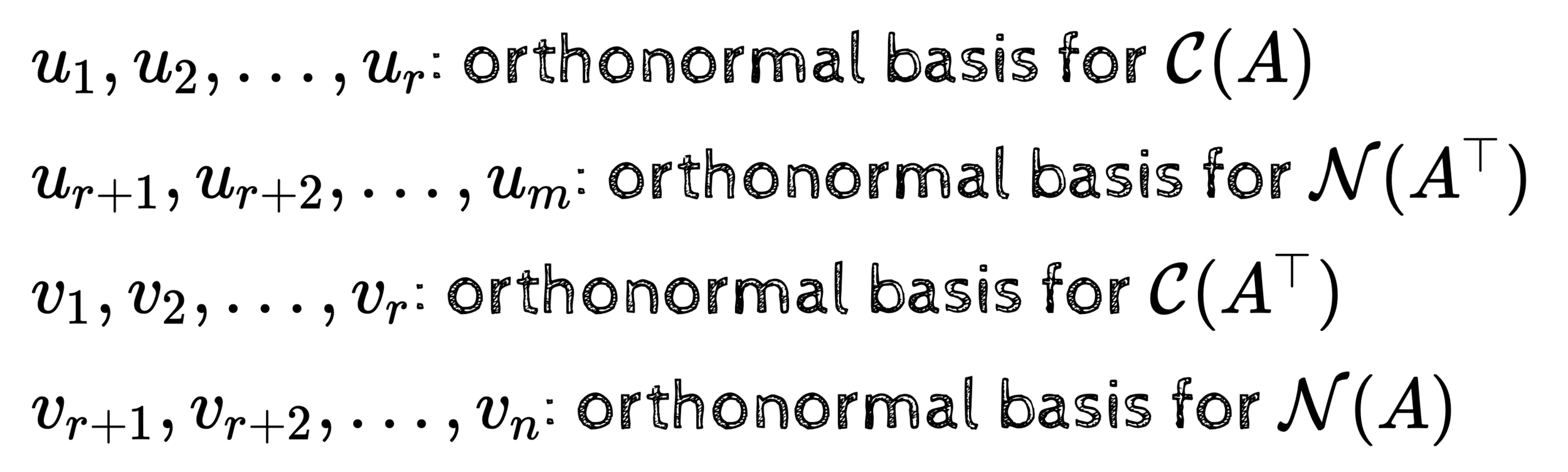
Let \(A_{m\times n}\) be a rank \(r\) matrix
\(\mathbf{u_1, u_2, \dots, u_r}\) be an orthonormal basis for \(\mathcal{C}(A)\)
\(\mathbf{u_{r+1}, u_{r+2}, \dots, u_{m}}\) be an orthonormal basis for \(\mathcal{N}(A^\top)\)
\(\mathbf{v_1, v_2, \dots, v_r}\) be an orthonormal basis for \(\mathcal{C}(A^\top)\)
\(\mathbf{v_{r+1}, v_{r+2}, \dots, v_{n}}\) be an orthonormal basis for \(\mathcal{N}(A)\)
Let \(A_{m\times n}\) be a rank \(r\) matrix
Fact 1: Such basis always exist
Fact 2: \(\mathbf{u_1, u_2, \dots, u_r, u_{r+1}, \dots, u_m}\) are orthonormal
In addition, we want
\(\mathbf{v_1, v_2, \dots, v_r, v_{r+1}, \dots, v_n}\) are orthonormal
A\mathbf{v_i} = \sigma_i\mathbf{u_i}~~\forall i\leq r
\therefore A
\begin{bmatrix}
\uparrow&\uparrow&\uparrow \\
\mathbf{v}_1&\dots&\mathbf{v}_r \\
\downarrow&\downarrow&\downarrow \\
\end{bmatrix}
=
\begin{bmatrix}
\uparrow&\uparrow&\uparrow \\
\mathbf{u}_1&\dots&\mathbf{u}_r \\
\downarrow&\downarrow&\downarrow \\
\end{bmatrix}
\begin{bmatrix}
\sigma_1&\dots&0 \\
0&\dots&0 \\
0&\dots&\sigma_r \\
\end{bmatrix}
The 4 fundamental subspaces: basis
A
\begin{bmatrix}
\uparrow&\uparrow&\uparrow \\
\mathbf{v}_1&\dots&\mathbf{v}_r \\
\downarrow&\downarrow&\downarrow \\
\end{bmatrix}
=
\begin{bmatrix}
\uparrow&\uparrow&\uparrow \\
\mathbf{u}_1&\dots&\mathbf{u}_r \\
\downarrow&\downarrow&\downarrow \\
\end{bmatrix}
\begin{bmatrix}
\sigma_1&\dots&0 \\
0&\dots&0 \\
0&\dots&\sigma_r \\
\end{bmatrix}
Finding \(U\) and \(V\)
\underbrace{A}_{m\times n}~\underbrace{V_r}_{n \times r} = \underbrace{U_r}_{m \times r}~\underbrace{\Sigma}_{r \times r}
(we don't know what such V and U are - we are just hoping that they exist)
\therefore A
\begin{bmatrix}
\uparrow&\uparrow&\uparrow&\uparrow&\uparrow \\
\mathbf{v}_1&\dots&\mathbf{v}_{r}&\mathbf{v}_{r+1}&\dots&\mathbf{v}_n \\
\downarrow&\downarrow&\downarrow&\downarrow&\downarrow \\
\end{bmatrix}=
\begin{bmatrix}
\uparrow&\uparrow&\uparrow&\uparrow&\uparrow&\uparrow \\
\mathbf{u}_1&\dots&\mathbf{u}_r&\mathbf{u}_{r+1}&\dots&\mathbf{u}_m \\
\downarrow&\downarrow&\downarrow&\downarrow&\downarrow&\downarrow \\
\end{bmatrix}
\begin{bmatrix}
\sigma_1&\dots&0&0&0 \\
0&\dots&0&0&0 \\
0&\dots&\sigma_r&0&0 \\
0&\dots&0&0&0 \\
0&\dots&0&0&0 \\
\end{bmatrix}
If \(V_r\) and \(U_r\) exist then
null space
First r columns of this product will be and the last n-r columns will be 0
n-r 0 colums
m-r 0 rows
\underbrace{A}_{m\times n}~\underbrace{V}_{n \times n} = \underbrace{U}_{m \times m}~\underbrace{\Sigma}_{m \times n}
\(V\) and \(U\) also exist
The last m-r columns of U will not contribute and hence the first r columns will be the same as and the last n-r columns will be 0
U_r \Sigma
AV_r
Finding \(U\) and \(V\)
AV=U\Sigma
A=U\Sigma V^\top
A^\top A=(U\Sigma V^\top)^\top U\Sigma V^\top
A^\top A=V\Sigma^\top U^\top U\Sigma V^\top
A^\top A=V\Sigma^\top\Sigma V^\top
diagonal
orthogonal
orthogonal
\(V\) is thus the matrix of the \(n\) eigen vectors of \(A^\top A\)
we know that this always exists because A'A is a symmetric matrix
AV=U\Sigma
A=U\Sigma V^\top
AA^\top =U\Sigma V^\top(U\Sigma V^\top)^\top
AA^\top =U\Sigma V^\top V\Sigma^\top U^\top
AA^\top=U\Sigma\Sigma^\top U^\top
diagonal
orthogonal
orthogonal
\(U\) is thus the matrix of the \(m\) eigen vectors of \(AA^\top \)
we know that this always exists because AA' is a symmetric matrix
\(\Sigma^\top\Sigma\) contains the eigenvalues of \(A^\top A \)
HW5:Prove that the non-0 eigenvalues of AA' and A'A are always equal
Finding \(U\) and \(V\)
\underbrace{A}_{m\times n} = \underbrace{U}_{m\times m}~\underbrace{\Sigma}_{m\times n}~\underbrace{V^\top}_{n\times n}
eigenvectors of AA'
transpose of the eigenvectors of A'A
square root of the eigenvalues of A'A or AA'
This is called the Singular Value Decomposition of \(A\)
\(\because U~and~V\) always exist, the SVD of any matrix \(A\) is always possible
since they are eigenvectors of a symmetric matrix
Some questions
\therefore A
\begin{bmatrix}
\uparrow&\uparrow&\uparrow&\uparrow&\uparrow \\
\mathbf{v}_1&\dots&\mathbf{v}_{r}&\mathbf{v}_{r+1}&\dots&\mathbf{v}_n \\
\downarrow&\downarrow&\downarrow&\downarrow&\downarrow \\
\end{bmatrix}=
\begin{bmatrix}
\uparrow&\uparrow&\uparrow&\uparrow&\uparrow&\uparrow \\
\mathbf{u}_1&\dots&\mathbf{u}_r&\mathbf{u}_{r+1}&\dots&\mathbf{u}_m \\
\downarrow&\downarrow&\downarrow&\downarrow&\downarrow&\downarrow \\
\end{bmatrix}
\begin{bmatrix}
\sigma_1&\dots&0&0&0 \\
0&\dots&0&0&0 \\
0&\dots&\sigma_r&0&0 \\
0&\dots&0&0&0 \\
0&\dots&0&0&0 \\
\end{bmatrix}
How do we know for sure that these \(\sigma s\) will be 0?
Recall: \(rank(A) = rank(A^\top A) = r\)
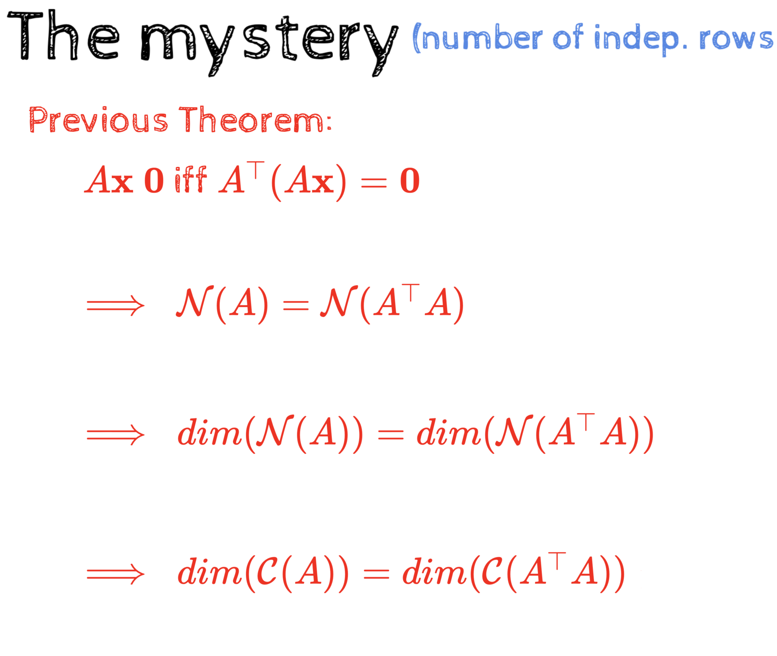
If \(rank(A) \lt n\) then rank \(A^\top A \lt n \implies A^\top A\) is singular
\(\implies A^\top A \) has 0 eigenvalues
How many?
as many as the dimension of the nullspace: \(n - r\)
Some questions
\therefore A
\begin{bmatrix}
\uparrow&\uparrow&\uparrow&\uparrow&\uparrow \\
\mathbf{v}_1&\dots&\mathbf{v}_{r}&\mathbf{v}_{r+1}&\dots&\mathbf{v}_n \\
\downarrow&\downarrow&\downarrow&\downarrow&\downarrow \\
\end{bmatrix}=
\begin{bmatrix}
\uparrow&\uparrow&\uparrow&\uparrow&\uparrow&\uparrow \\
\mathbf{u}_1&\dots&\mathbf{u}_r&\mathbf{u}_{r+1}&\dots&\mathbf{u}_m \\
\downarrow&\downarrow&\downarrow&\downarrow&\downarrow&\downarrow \\
\end{bmatrix}
\begin{bmatrix}
\sigma_1&\dots&0&0&0 \\
0&\dots&0&0&0 \\
0&\dots&\sigma_r&0&0 \\
0&\dots&0&0&0 \\
0&\dots&0&0&0 \\
\end{bmatrix}
How do we know that these form a basis for the column space of A?
How do we know that these form a basis for the rowspace of A?
\underbrace{~~~~~~~~~~~~~~~~~~~~~~~~~~~~~~}
\underbrace{~~~~~~~~~~~~~~~~~~~~~~~~~~~~~~}
so far we only know that these are the eigenvectors of AA'
so far we only know that these are the eigenvectors of A'A
Please work this out! You really need to see this on your own! HW5
Why do we care about SVD?
A=U\Sigma V^\top
\therefore A=
\begin{bmatrix}
\uparrow&\uparrow&\uparrow&\uparrow&\uparrow \\
\mathbf{u}_1&\dots&\mathbf{u}_r&\dots&\mathbf{u}_m \\
&\\
&\\
\downarrow&\downarrow&\downarrow&\downarrow&\downarrow\\
\end{bmatrix}
\begin{bmatrix}
\sigma_1&\dots&0&0&0&0 \\
0&\dots&0&0&0&0 \\
0&\dots&\sigma_r&0&0&0 \\
0&\dots&0&0&0&0 \\
0&\dots&0&0&0&0 \\
\end{bmatrix}
\begin{bmatrix}
\leftarrow&\dots&\mathbf{v}_{1}^\top&\cdots&\dots&\rightarrow \\
&\\
\leftarrow&\dots&\mathbf{v}_{r}^\top&\cdots&\dots&\rightarrow \\
&\\
&\\
\leftarrow&\dots&\mathbf{v}_{n}^\top&\cdots&\dots&\rightarrow \\
\end{bmatrix}
\therefore A=
\begin{bmatrix}
\uparrow&\uparrow&\uparrow&\uparrow&\uparrow \\
\sigma_1\mathbf{u}_1&\dots&\sigma_r\mathbf{u}_r&\dots&0 \\
&\\
&\\
\downarrow&\downarrow&\downarrow&\downarrow&\downarrow\\
\end{bmatrix}
\begin{bmatrix}
\leftarrow&\dots&\mathbf{v}_{1}^\top&\cdots&\dots&\rightarrow \\
&\\
\leftarrow&\dots&\mathbf{v}_{r}^\top&\cdots&\dots&\rightarrow \\
&\\
&\\
\leftarrow&\dots&\mathbf{v}_{n}^\top&\cdots&\dots&\rightarrow \\
\end{bmatrix}
\therefore A=\sigma_1\mathbf{u_1}\mathbf{v_1}^\top+\sigma_2\mathbf{u_2}\mathbf{v_2}^\top+\cdots+\sigma_r\mathbf{u_r}\mathbf{v_r}^\top
n-r 0 columns
Why do we care about SVD?
A=U\Sigma V^\top
\therefore A=\sigma_1\mathbf{u_1}\mathbf{v_1}^\top+\sigma_2\mathbf{u_2}\mathbf{v_2}^\top+\cdots+\sigma_r\mathbf{u_r}\mathbf{v_r}^\top
largest sigma
smallest sigma
we can sort these terms according to sigmas
\(A\) has \(m \times n \) elements
Each \(\mathbf{u_i}\) has m elements
Each \(\mathbf{v_i}\) has n elements
After SVD you can represent \(A\) using \(r(m+n+1)\) elements
If the rank is very small then this would lead to significant compression
Even further compression can be obtained by throwing away terms corresponding to vert small \(\sigma s\)
Fun with flags :-)

Original Image: 1200 x 800
Lot of redundancy
\(rank \lt\lt 800\)

Original Image: 1200 x 800
Lot of redundancy
\(rank \lt\lt 800\)
Puzzle: What is the rank of this flag?
Best rank-k approximation
||A||_F = \sqrt{\sum_{i=1}^m\sum_{j=1}^n |A_{ij}|^2}
A=\sigma_1\mathbf{u_1}\mathbf{v_1}^\top+\sigma_2\mathbf{u_2}\mathbf{v_2}^\top+\cdots+\sigma_k\mathbf{u_k}\mathbf{v_k}^\top+\cdots+\sigma_r\mathbf{u_r}\mathbf{v_r}^\top
Frobenius norm
\hat{A}_k=\sigma_1\mathbf{u_1}\mathbf{v_1}^\top+\sigma_2\mathbf{u_2}\mathbf{v_2}^\top+\cdots+\sigma_k\mathbf{u_k}\mathbf{v_k}^\top
rank-k approximation of A - dropped the last r - k terms
Theorem: SVD gives the best rank-\(k\) approximation of the matrix \(A\)
i.e. \(||A - \hat{A}_k||_F\) is minimum when
\hat{A}_k=U_k\Sigma_kV^T_k
we will not prove this
Summary of the course
(in 3 pictures)
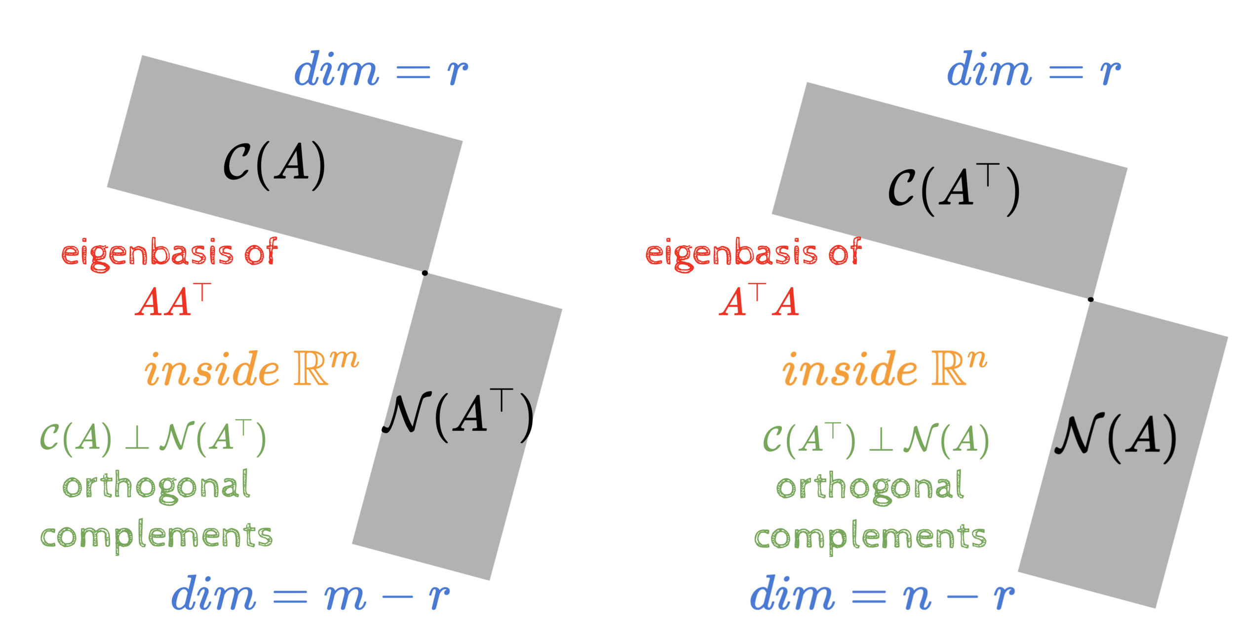
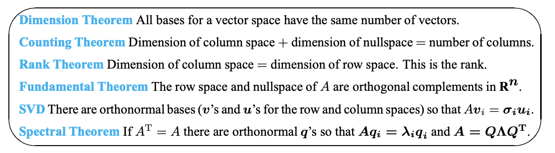
Summary of the course
(in 6 great theorems)
Source: Introduction to Linear Algebra, Prof. Gilbert Strang
The full story
(How would you do this in practice?)
Compute the n eigen vectors of X TX
Sort them according to the corresponding eigenvalues
Retain only those eigenvectors corresponding to the top-k eigenvalues
Project the data onto these k eigenvectors
We know that n such vectors will exist since it is a symmetric matrix
These are called the principal components
Heuristics: k=50,100 or choose k such that λk/λmax > t
Copy of Copy of CS6015: Lecture 21
By Madhura Pande cs17s031
Copy of Copy of CS6015: Lecture 21
Lecture 21: Principal Component Analysis (the math)


