Spurious self-feedback in infection models
Claudia Merger, Jasper Albers,
Carsten Honerkamp, Moritz Helias

Spread of disease: Models
- Markov process
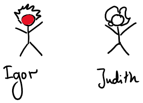
- Population: Susceptible, Infected, Recovered/Removed


Self-feedback
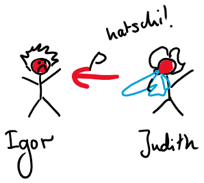
Self-feedback in SIS model
More information: Pastor-Satorras et. al., A. Epidemic processes in complex networks. Rev. Mod. Phys. 87, 925–979 (2015).
t = 0 \\
x_i(t)= \begin{pmatrix} 0\\ 1 \end{pmatrix}, \, x_j(t)= \begin{pmatrix} 1\\ 0 \end{pmatrix}
S_i(t)= 1 \quad \text{susceptible} \\
I_i(t)= 1 \quad \text{infected} \\
x_i(t) = \begin{pmatrix}
S_i(t) \\
I_i(t)
\end{pmatrix}
Self-feedback in SIS model
More information: Pastor-Satorras et. al., A. Epidemic processes in complex networks. Rev. Mod. Phys. 87, 925–979 (2015).
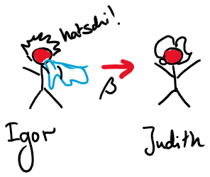
t = 0 \\
x_i(t)= \begin{pmatrix} 0\\ 1 \end{pmatrix}, \, x_j(t)= \begin{pmatrix} 1\\ 0 \end{pmatrix}
t = 1 \\
x_i(t)= \begin{pmatrix} 0\\ 1 \end{pmatrix}, \, x_j(t)= \begin{pmatrix} 0\\ 1
\end{pmatrix}
t = 2 \\
x_i(t)= \begin{pmatrix} 0\\ 0 \end{pmatrix}, \, x_j(t)= \begin{pmatrix} 0\\ 1
\end{pmatrix}
S_i(t)= 1 \quad \text{susceptible} \\
I_i(t)= 1 \quad \text{infected} \\
x_i(t) = \begin{pmatrix}
S_i(t) \\
I_i(t)
\end{pmatrix}
Self-feedback in SIS model
More information: Pastor-Satorras et. al., A. Epidemic processes in complex networks. Rev. Mod. Phys. 87, 925–979 (2015).
t = 0 \\
x_i(t)= \begin{pmatrix} 0\\ 1 \end{pmatrix}, \, x_j(t)= \begin{pmatrix} 1\\ 0 \end{pmatrix}
t = 1 \\
x_i(t)= \begin{pmatrix} 0\\ 1 \end{pmatrix}, \, x_j(t)= \begin{pmatrix} 0\\ 1
\end{pmatrix}
t = 2 \\
x_i(t)= \begin{pmatrix} 0\\ 0 \end{pmatrix}, \, x_j(t)= \begin{pmatrix} 0\\ 1
\end{pmatrix}
t = 3 \\
x_i(t)= \begin{pmatrix} 0\\ 1 \end{pmatrix}, \, x_j(t)= \begin{pmatrix} 0\\ 1
\end{pmatrix}
S_i(t)= 1 \quad \text{susceptible} \\
I_i(t)= 1 \quad \text{infected} \\
x_i(t) = \begin{pmatrix}
S_i(t) \\
I_i(t)
\end{pmatrix}
Self-feedback in SIR model
S_i(t)= 1 \quad \text{susceptible} \\
I_i(t)= 1 \quad \text{infected} \\
x_i(t) = \begin{pmatrix}
S_i(t) \\
I_i(t)
\end{pmatrix}
Self-feedback in SIR model
t = 0 \\
x_i(t)= \begin{pmatrix} 0\\ 1 \end{pmatrix}, \, x_j(t)= \begin{pmatrix} 1\\ 0 \end{pmatrix}
t = 1 \\
x_i(t)= \begin{pmatrix} 0\\ 1 \end{pmatrix}, \, x_j(t)= \begin{pmatrix} 0\\ 1
\end{pmatrix}
Self-feedback is forbidden!
S_i(t)= 1 \quad \text{susceptible} \\
I_i(t)= 1 \quad \text{infected} \\
x_i(t) = \begin{pmatrix}
S_i(t) \\
I_i(t)
\end{pmatrix}
Self-feedback in SIR model
t = 0 \\
x_i(t)= \begin{pmatrix} 0\\ 1 \end{pmatrix}, \, x_j(t)= \begin{pmatrix} 1\\ 0 \end{pmatrix}
t = 1 \\
x_i(t)= \begin{pmatrix} 0\\ 1 \end{pmatrix}, \, x_j(t)= \begin{pmatrix} 0\\ 1
\end{pmatrix}
t = 2 \\
x_i(t)= \begin{pmatrix} 0\\ 0 \end{pmatrix}, \, x_j(t)= \begin{pmatrix} 0\\ 1
\end{pmatrix}
t = 3 \\
x_i(t)= \begin{pmatrix} 0\\ 1 \end{pmatrix}, \, x_j(t)= \begin{pmatrix} 0\\ 1
\end{pmatrix}
Self-feedback is forbidden!
S_i(t)= 1 \quad \text{susceptible} \\
I_i(t)= 1 \quad \text{infected} \\
x_i(t) = \begin{pmatrix}
S_i(t) \\
I_i(t)
\end{pmatrix}

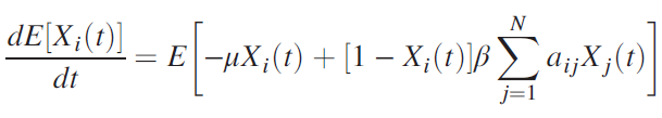
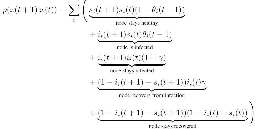
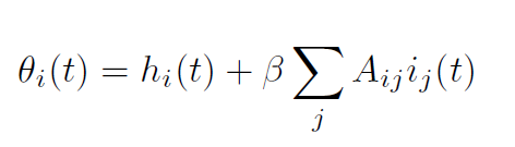
Average dynamics
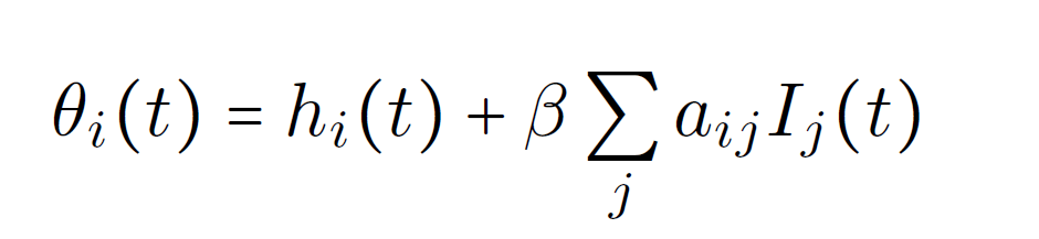
input field \(\theta_i\) for each node \(i\)
expectation values
\(\rho^{S}_i(t)=\langle S_i(t) \rangle \)
\(\rho^{I}_i(t)=\langle I_i(t) \rangle \)
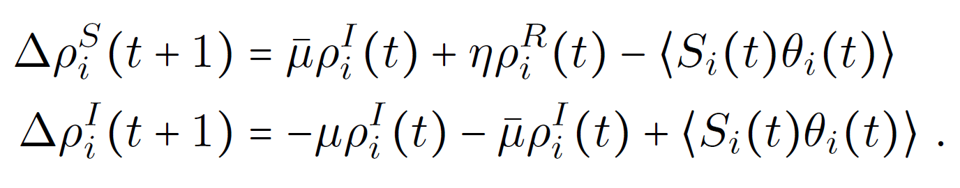
Mean-field equations
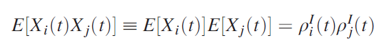
\langle S_i(t) \theta_i(t) \rangle \approx \langle S_i(t) \rangle \langle \theta_i(t) \rangle
Mean-field equations
\langle S_i(t) \theta_i(t) \rangle \approx \langle S_i(t) \rangle \langle \theta_i(t) \rangle
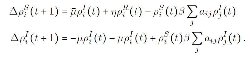
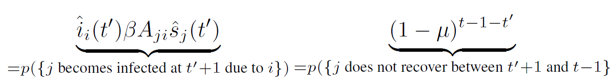
this approximation artificially introduces self-feedback
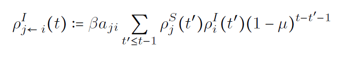
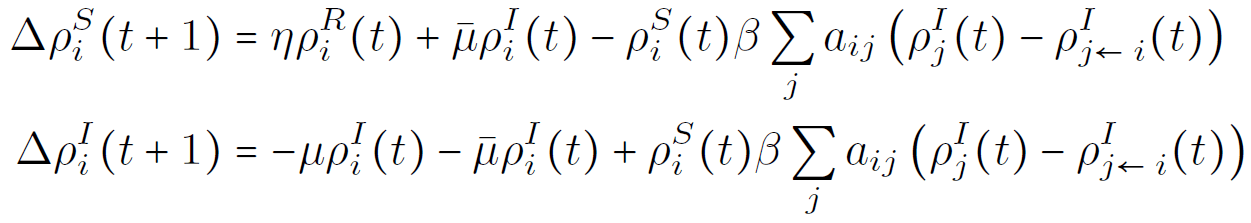
Mean-field equations
this approximation artificially introduces self-feedback
= \dots + \beta a_{ji} \rho^I_i (t-1)
Self-feedback is a second order effect
\propto \beta^2 \text{ correction}
We compute second order corrections
Roudi, Y. & Hertz, J. Dynamical TAP equations for non-equilibrium Ising spin glasses. Journal of Statistical Mechanics: Theory and Experiment 2011, P03031 (2011).
Simulation with NEST
Difficulty: Spiking neurons \( \rightarrow \) neurons with 3 discrete states
basis for implementation: binary neurons
idea: communicate changes to \( \theta_i \)
signal change of state via spikes:
Spike with multiplicity 1: \( S \rightarrow I \)
Spike with multiplicity 2: \( I \rightarrow S,R \)
Simulation with NEST
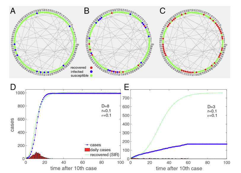
Results
SIR model
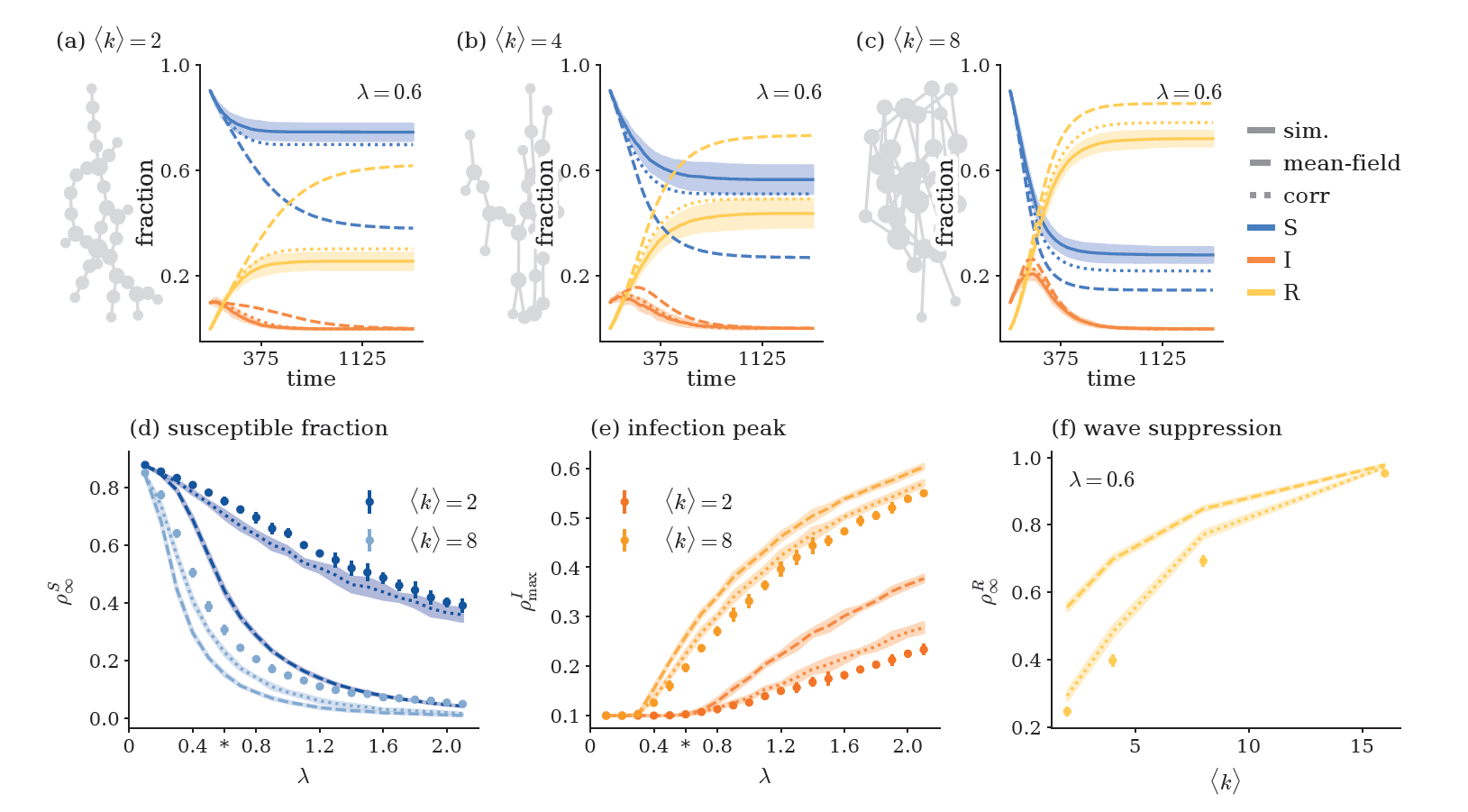
SIR model
\( \Rightarrow \) Sparsity suppresses activity!
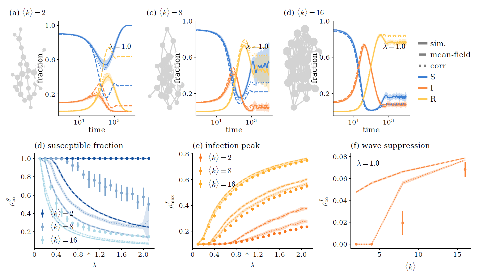
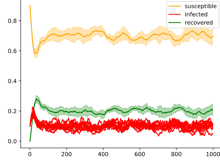
SIRS & SIS model
same corrections even though self-feedback is allowed.
only partial cancellation
SIRS & SIS model
same corrections even though self-feedback is allowed.
only partial cancellation
SIRS model
State with finite endemic activity exists,
but at which \( \lambda=\frac{\beta}{\mu} \) ?
SIRS model
State with finite endemic activity exists,
but at which \( \lambda=\frac{\beta}{\mu} \) ?
\( \Rightarrow \) Linearize around \( \rho^I =0\) and check when \(\Delta \rho^I >0 \)
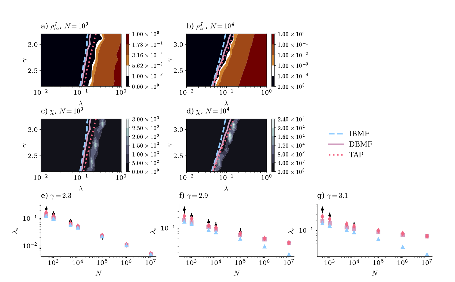
SIRS model
State with finite endemic activity exists,
but at which \( \lambda=\frac{\beta}{\mu} \) ?
\( \Rightarrow \) Linearize around \( \rho^I =0\) and check when \(\Delta \rho^I >0 \)
Mean-field: \(\lambda_c^{-1} = \lambda_a^{max} \)
\(a= \) adjacency matr.
SIRS model
State with finite endemic activity exists,
but at which \( \lambda=\frac{\beta}{\mu} \) ?
\( \Rightarrow \) Linearize around \( \rho^I =0\) and check when \(\Delta \rho^I >0 \)
Mean-field: \(\lambda_c^{-1} = \lambda_a^{max} \)
corrected equation:
\( \lambda_c^{-1} = \lambda_D^{max} \)
\(a= \) adjacency matr.
D =
\begin{pmatrix}
a & -1 \\
K & 0
\end{pmatrix} \\
K_{ij} = \delta_{ij} \text{degree}_i
\rho_{\infty}^I
Mean-field: \(\lambda_c^{-1} = \lambda_a^{max} \)
corrected equation:
\( \lambda_c^{-1} = \lambda_D^{max} \)
\text{scale free networks}: \\
p(\text{degree}) \sim (\text{degree})^{-\gamma}
Mean-field: \(\lambda_c^{-1} = \lambda_a^{max} \)
corrected equation:
\( \lambda_c^{-1} = \lambda_D^{max} \)
\text{scale free networks}: \\
p(\text{degree}) \sim (\text{degree})^{-\gamma}
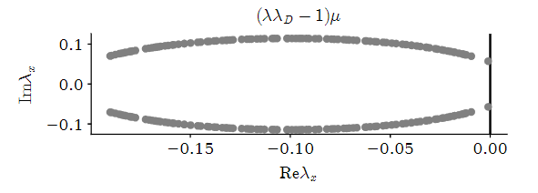
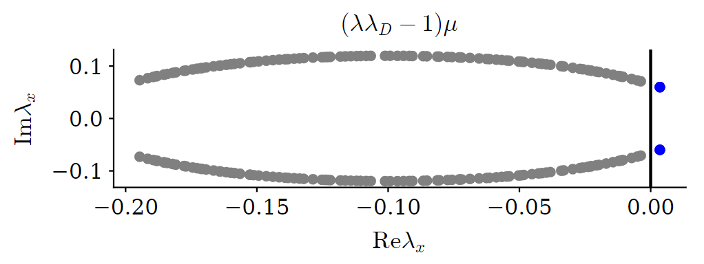
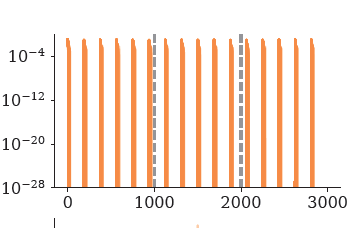
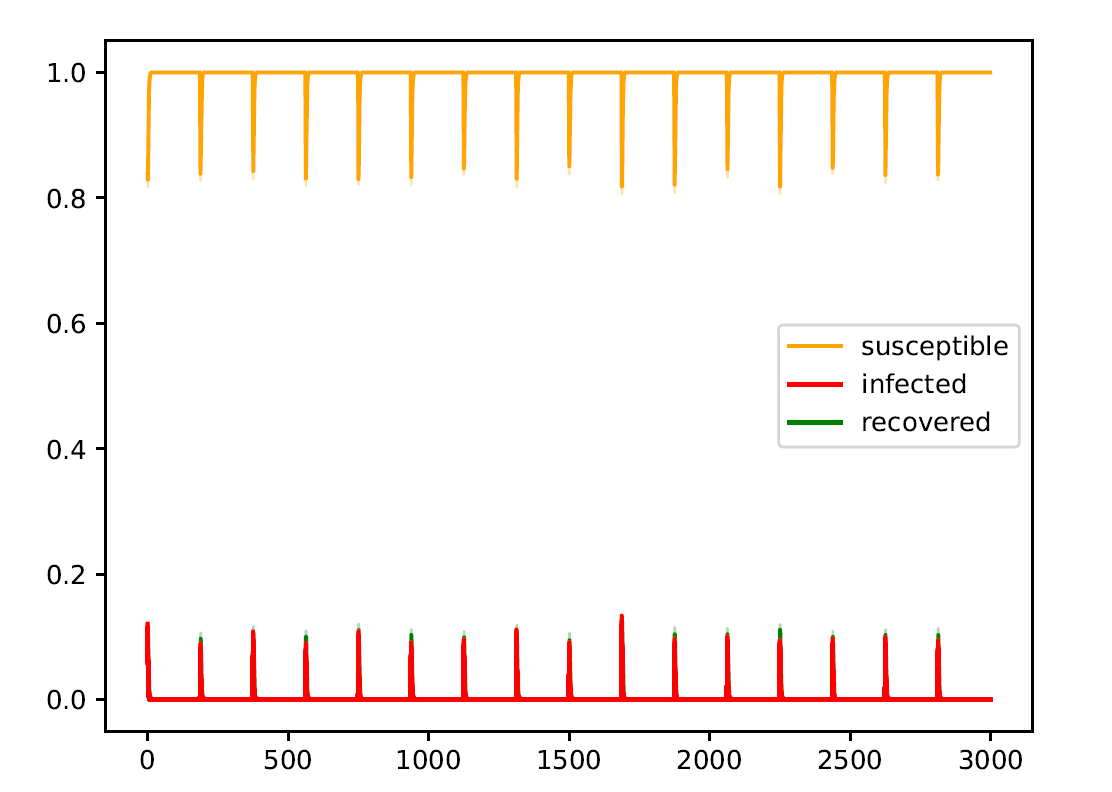
Oscillations?
corrected equation:
\(\Delta \rho^I = \left( \lambda \lambda_D^{max} -1 \right) \mu \rho^I \)
D =
\begin{pmatrix}
a & -1 \\
K & 0
\end{pmatrix} \\
K_{ij} = \delta_{ij} \text{degree}_i
Imaginary leading eigenvalues \( \lambda_D^{max} \) ?!
Yes, for special network architectures
Oscillations?
corrected equation:
\(\Delta \rho^I = \left( \lambda \lambda_D^{max} -1 \right) \mu \rho^I \)
Random Regular Networks with \(\langle k \rangle = 3\)
(all nodes have equal degree, connections random)
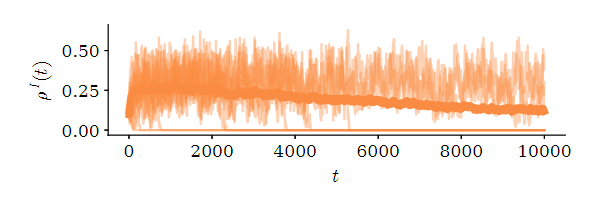
\lambda=0.66
\lambda=0.69
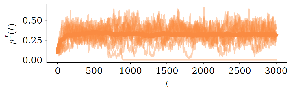
Oscillations?
corrected equation:
\(\Delta \rho^I = \left( \lambda \lambda_D^{max} -1 \right) \mu \rho^I \)
Random Regular Networks with \(\langle k \rangle = 3\)
(all nodes have equal degree, connections random)
\lambda=0.66
\lambda=0.69
Oscillations?
corrected equation:
\(\Delta \rho^I = \left( \lambda \lambda_D^{max} -1 \right) \mu \rho^I \)
D =
\begin{pmatrix}
a & -1 \\
K & 0
\end{pmatrix} \\
K_{ij} = \delta_{ij} \text{degree}_i
time
pop. fraction
Imaginary eigenvalues?!
Yes, for special network architectures
Random Regular Networks
(all nodes have equal degree, connections random)
Summary & Outlook:
- Self-feedback plays an important role in non-equilibrium processes on networks
- Using path integral formulations, we find that self-feedback cancels for the SIR model (partially)
- Corrections to SIRS model also cancel self-feedback (partially)
Open questions and To-Dos
- Frequency of oscillations in random regular or Erdös-Renyi type networks
- difference between SIS & SIRS networks?
Oscillations: Problems
When setting "num_threads" >1:
\rho^I
\text{time}
\beta
\beta
\beta

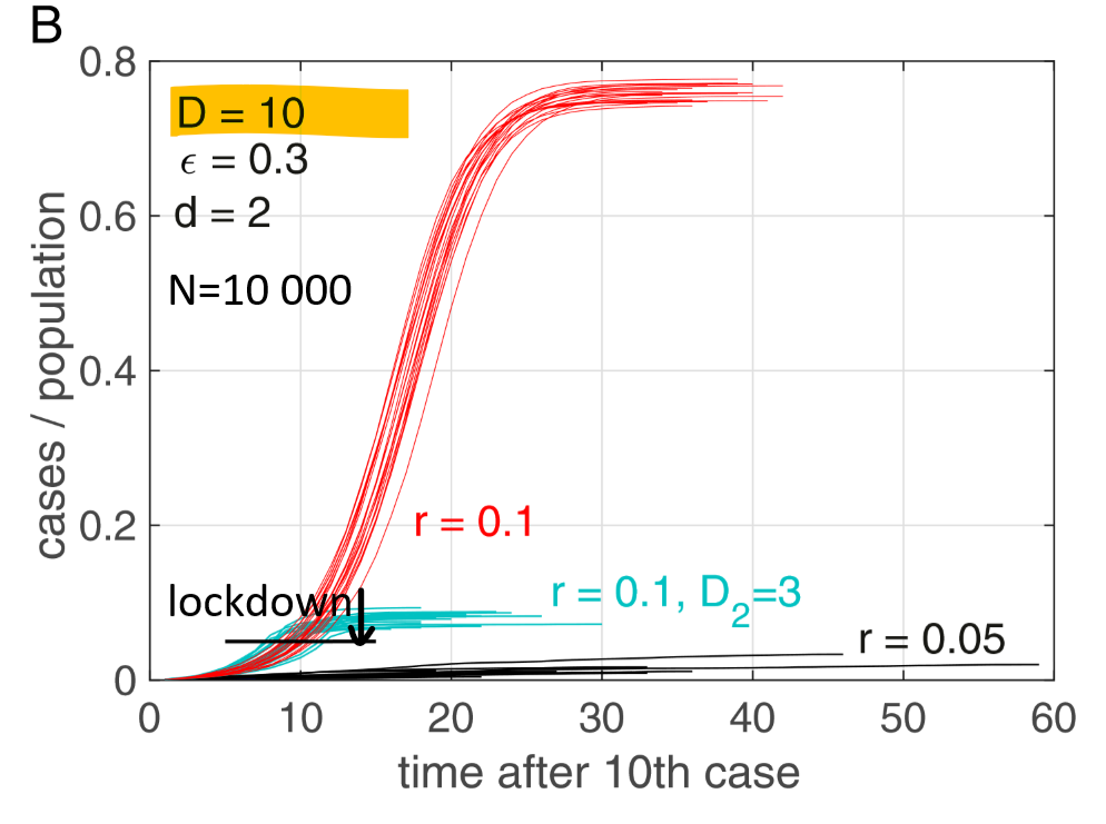
S-shaped growth vs. linear growth
S-shaped growth vs. linear growth
\beta
\beta
\beta
Change in or degree
Change in inf. dynamics
\beta
However: Here, meanfield is done only in population average \( \hat{s}_i \approx \hat{s} \)
Main questions:
Dynamics explained by...
- Architecture and mean-field?
- Fluctuation corrections?
A_{ij}
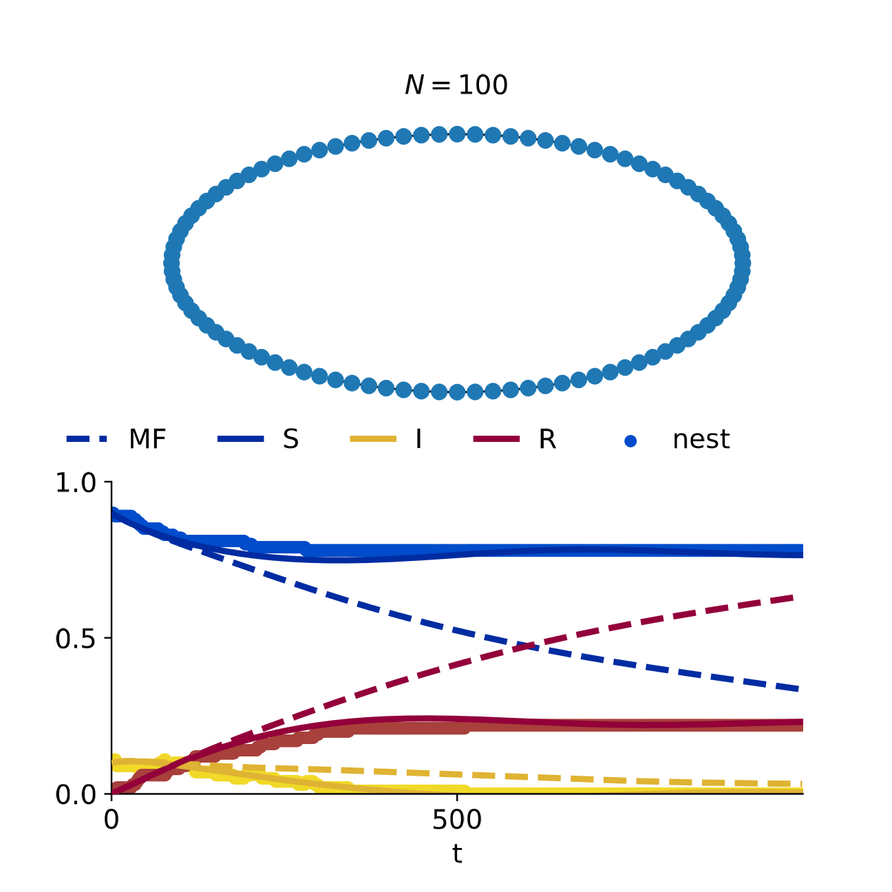
Experiment: Linear Chain, individual-based.
Mean-field overestimates inf. dynamics even if network architecture is accounted for!
More literature on SIR model
-
Moein, S., Nickaeen, N., Roointan, A. et al. Inefficiency of SIR models in forecasting COVID-19 epidemic: a case study of Isfahan. Sci Rep 11, 4725 (2021). https://doi.org/10.1038/s41598-021-84055-6
- Differential equation meanfield form of SIR model does not predict spread of disease well.
-
Lazzizzera I. The SIR model towards the data: One year of Covid-19 pandemic in Italy case study and plausible "real" numbers. Eur Phys J Plus. 2021;136(8):802. doi: 10.1140/epjp/s13360-021-01797-y. Epub 2021 Aug 4. PMID: 34377623; PMCID: PMC8336674.
- meanfield SIR model fits data if recovery curve is multiplied by 3.
-
B. Malavika, S. Marimuthu, Melvin Joy, Ambily Nadaraj, Edwin Sam Asirvatham, L. Jeyaseelan, Forecasting COVID-19 epidemic in India and high incidence states using SIR and logistic growth models, Clinical Epidemiology and Global Health,
- "Invariably, the SIR model overestimates the active number of cases."
Self-feedback in SIS model
X_i = 0 \, \rightarrow \, \text{susceptible} \\
X_i = 1 \, \rightarrow \, \text{infected}
E \left[ X_i(t) \right] := \rho_i(t), \\
\text{prb. } X_i(t) \text{ infected at time } t
\text{mean-field approx:}
\text{mean-field update:}
More information: Pastor-Satorras et. al., A. Epidemic processes in complex networks. Rev. Mod. Phys. 87, 925–979 (2015).
Self-feedback in SIS model
More information: Pastor-Satorras et. al., A. Epidemic processes in complex networks. Rev. Mod. Phys. 87, 925–979 (2015).
t = 0 \\
X_i = 1, \, X_j = 0
Self-feedback in SIS model
More information: Pastor-Satorras et. al., A. Epidemic processes in complex networks. Rev. Mod. Phys. 87, 925–979 (2015).
t = 0 \\
X_i = 1, \, X_j = 0
t = 1 \\
X_i = 1, \, X_j = 1
Self-feedback in SIS model
More information: Pastor-Satorras et. al., A. Epidemic processes in complex networks. Rev. Mod. Phys. 87, 925–979 (2015).
t = 0 \\
X_i = 1, \, X_j = 0
t = 1 \\
X_i = 1, \, X_j = 1
t = 2 \\
X_i = 0, \, X_j = 1

Self-feedback in SIS model
More information: Pastor-Satorras et. al., A. Epidemic processes in complex networks. Rev. Mod. Phys. 87, 925–979 (2015).
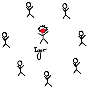
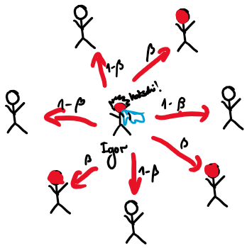
Self-feedback is strongest for hubs!
Castellano C, et. al. Cumulative Merging Percolation and the Epidemic Transition of the Susceptible-Infected-Susceptible Model in Networks. Phys Rev X. 2020 Jan 1;10(1):011070. doi: 10.1103/PhysRevX.10.011070.
t = 0 \\
X_i = 1, \, X_j = 0
t = 1 \\
X_i = 1, \, X_j = 1
t = 2 \\
X_i = 0, \, X_j = 1
t = 3 \\
X_i = 1, \, X_j = 1
Self-feedback in SIS model
X_i = 0 \, \rightarrow \, \text{susceptible} \\
X_i = 1 \, \rightarrow \, \text{infected}
E \left[ X_i(t) \right] := \rho_i(t), \\
\text{prb. } X_i(t) \text{ infected at time } t
Self-feedback in SIS model
X_i = 0 \, \rightarrow \, \text{susceptible} \\
X_i = 1 \, \rightarrow \, \text{infected}
E \left[ X_i(t) \right] := \rho_i(t), \\
\text{prb. } X_i(t) \text{ infected at time } t
Corrected update equations:
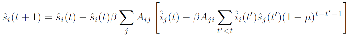
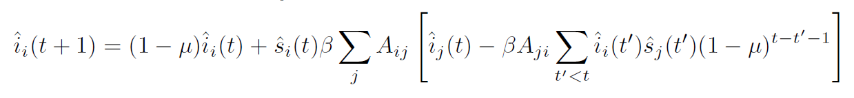
mean-field
mean-field
flu. correction / "TAP term"
flu. correction / "TAP term"
Corrected update equations:
mean-field
mean-field
flu. correction / "TAP term"
flu. correction / "TAP term"
Corrected update equations:
Correction cancels self-feedback!
t = 0 \\
x_i(t)= \begin{pmatrix} 0\\ 1 \end{pmatrix}, \, x_j(t)= \begin{pmatrix} 1\\ 0 \end{pmatrix}
t = 1 \\
x_i(t)= \begin{pmatrix} 0\\ 1 \end{pmatrix}, \, x_j(t)= \begin{pmatrix} 0\\ 1
\end{pmatrix}
t = 2 \\
x_i(t)= \begin{pmatrix} 0\\ 0 \end{pmatrix}, \, x_j(t)= \begin{pmatrix} 0\\ 1
\end{pmatrix}
t = 3 \\
x_i(t)= \begin{pmatrix} 0\\ 1 \end{pmatrix}, \, x_j(t)= \begin{pmatrix} 0\\ 1
\end{pmatrix}
mean-field
mean-field
flu. correction / "TAP term"
flu. correction / "TAP term"
SIR model
Analogous 2-state problem:
Roudi, Y. & Hertz, J. Dynamical TAP equations for non-equilibrium Ising spin glasses. Journal of Statistical Mechanics: Theory and Experiment 2011, P03031 (2011).
update probability:
Compute second order corrections!
Analogous 2-state problem:
Roudi, Y. & Hertz, J. Dynamical TAP equations for non-equilibrium Ising spin glasses. Journal of Statistical Mechanics: Theory and Experiment 2011, P03031 (2011).
update probability:
Compute second order corrections!
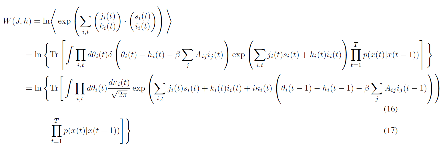
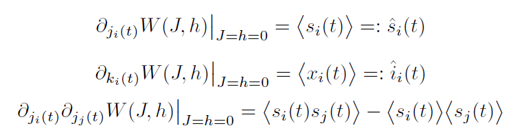
Cumulant generating functon
Compute second order corrections!
Cumulant generating functon
Compute second order corrections!
Cumulant generating functon
Compute second order corrections!
Cumulant generating functon
Compute second order corrections!
Cumulant generating functon
Effective action: Legendre transform

Effective action: Legendre transform
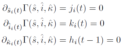
eq. of state
Effective action: Legendre transform
eq. of state
mean-field
flu. correction / "TAP term"
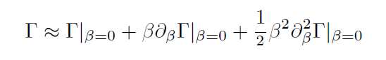
Plefka expansion: Expansion in \( \beta \)
Copy of Fluctuation corrections for SIR model
By merger


