Massively parallel implementation in Python of a pseudo-spectral DNS code for turbulent flows

Assoc. Professor Mikael Mortensen

Department of Mathematics, University of Oslo

Center for Biomedical Computing, Simula Research Laboratory

KAUST

4/5 - 2016

Direct Numerical Simulations of turbulence are performed with low-level Fortran or C

3D + time and HUGE resolution

Serious number crunching - extreme computing

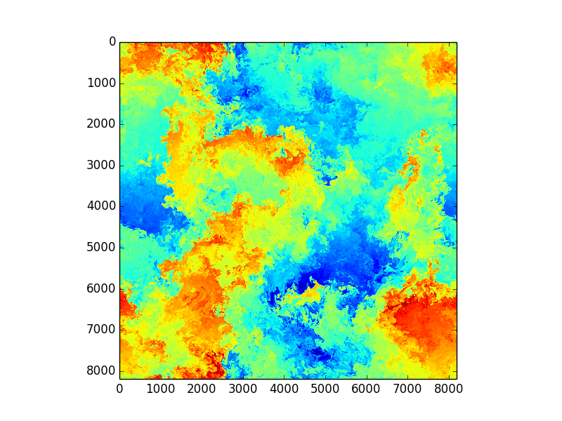
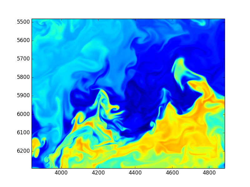
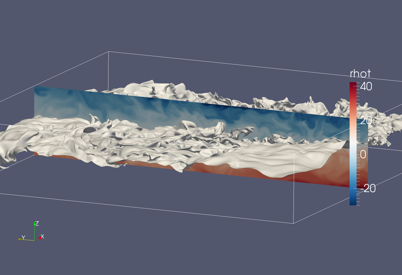
Images from huge DNS simulations by S. de Bruyn Kops, UmassAmherst, College of Engineering

Is it possible to write a competitive, state of the art turbulence solver in Python?

From scratch?

(Not just wrapping a Fortran solver)

Using only numpy/scipy/mpi4py?

Can this solver run on thousands of cores?

With billions of unknowns?

As fast as C?

Turns out 100 lines of Python code can get you almost there!

Turbulence is governed by the Navier Stokes equations

Triply periodic domain

Fourier space

Navier Stokes in spectral space

Eliminate pressure and solve ODEs:

Pseudo-spectral treatment of nonlinearity

Explicit timestepping (4th order Runge-Kutta)

Classical pseudo-spectral Navier-Stokes solver

The kind that has been used to break records since the day of the first supercomputer

Implementation

A few computational details

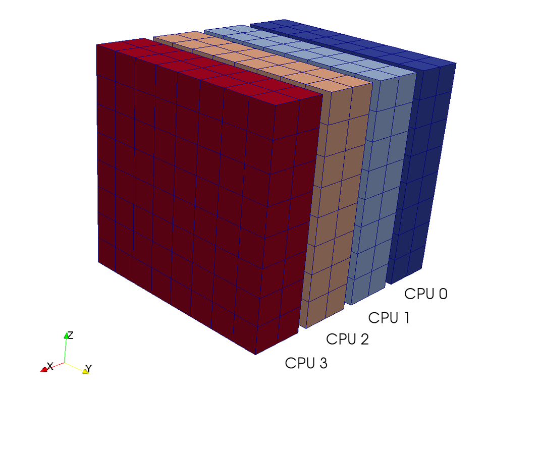
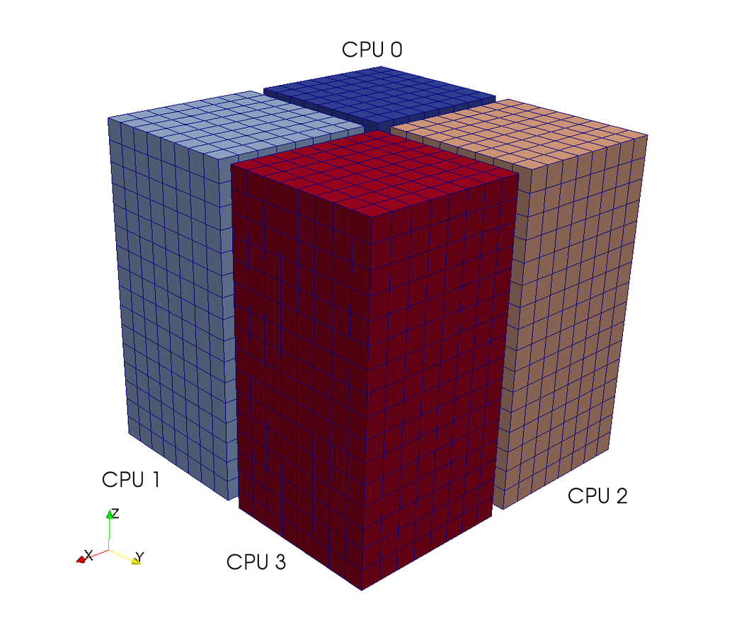
A computational box (mesh) needs to be distributed between a (possibly) large number of processors

N^3, N \sim 1000 - 10000

N^3, N \sim 1000 - 10000

Mesh size:

Pencil

Slab

\le N^2

\le N^2

CPUs

\le N

\le N

CPUs

mpi4py

by Licandro Dalcin at KAUST

Wraps almost the entire MPI library and handles distribution of numpy arrays at the speed of C

from mpi4py import MPI
comm = MPI.MPI_COMM_WORLD
print "Hello Licandro from rank", comm.Get_rank()

>>> mpirun -np 1000 python HelloLicandro.py

Hello Licandro from rank 0
Hello Licandro from rank 1
Hello Licandro from rank 3
...

MPI is basically needed to do 3D forward and backward FFT

and some postprocessing

HelloLicandro.py:

3D FFT with MPI

Slab decomposition (max N CPUs)

There are a few low level 3D FFT modules with MPI (e.g., libfftw, P3DFFT) but none that have been wrapped or is easily called from python

Need to adapt single core FFT

(numpy.fft, scipy.fftpack, pyfftw)

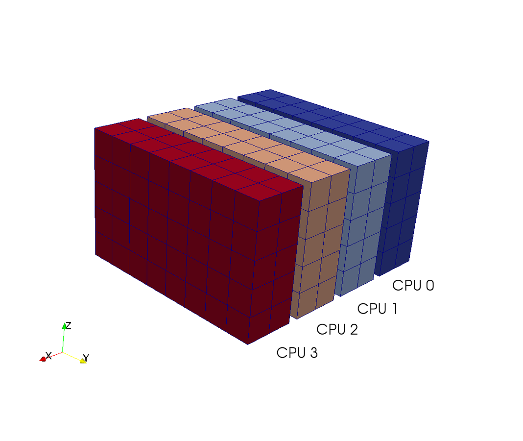
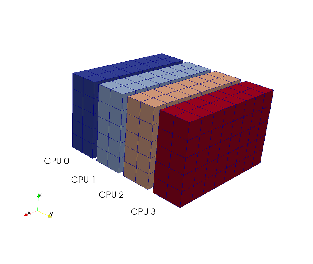
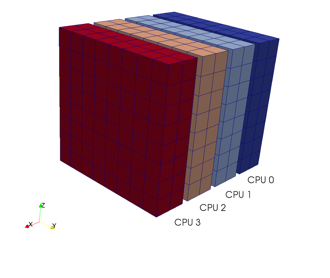
3D FFT with MPI

in a nutshell

real FFT in z, complex in y

No MPI required

Transpose and distribute

Then FFT in last direction

2D FFTs in Y-Z planes (local)
transpose operation
distribute data (MPI Alltoall)
FFT in X-direction

What does it really take?

Done!

3D FFT with MPI

in a nutshell

import numpy
from mpi4py import MPI

comm = MPI.COMM_WORLD
num_processes = comm.Get_size()

# Consider a problem of global size (N, N, N)
N = 128                # Must be power of 2
Np = N / num_processes # Decomposition - each process has Np items along x-direction

# Declare some work arrays used for the transform (could be done without Uc_hatT)
Uc_mpi  = numpy.zeros((num_processes, Np, Np, N/2+1), complex)
Uc_hatT = numpy.zeros((Np, N, N/2+1), complex)
def rfftn_mpi(u, fu):
    """3D FFT with MPI"""
    Uc_hatT[:] = numpy.fft.rfft2(u, axes=(1,2))                                   # 1!
    Uc_mpi[:] = numpy.rollaxis(Uc_hatT.reshape(Np, num_processes, Np, N/2+1), 1)  # 2!
    comm.Alltoall([Uc_mpi, MPI.F_DOUBLE_COMPLEX], [fu, MPI.F_DOUBLE_COMPLEX])     # 3!
    fu[:] = numpy.fft.fft(fu, axis=0)                                             # 4!
    return fu

# Create a variable U(N, N, N), distributed along first index
U = numpy.random.random((Np, N, N))
U_hat = numpy.zeros((N, Np, N/2+1), complex) # This is the transform

# Perform transform
U_hat = rfftn_mpi(U, U_hat)

# Now do the inverse
Uc_hat  = numpy.zeros_like(U_hat) # Intermediate work array

def irfftn_mpi(fu, u):
    """Inverse 3D FFT (irfftn) with MPI"""
    Uc_hat[:] = numpy.fft.ifft(fu, axis=0)                                        # 1!
    comm.Alltoall([Uc_hat, MPI.F_DOUBLE_COMPLEX], [Uc_mpi, MPI.F_DOUBLE_COMPLEX]) # 2!
    Uc_hatT[:] = numpy.rollaxis(Uc_mpi, 1).reshape(Uc_hatT.shape)                 # 3!
    u[:] = numpy.fft.irfft2(Uc_hatT, axes=(1,2))                                  # 4!
    return u

U_copy = numpy.zeros_like(U)
U_copy = irfftn_mpi(U_hat, U_copy)
assert numpy.allclose(U_copy, U)

real FFT in z, complex in y

No MPI required

Transpose and distribute

Then FFT in last direction

4 steps!

How many lines of code in C++/Fortran?

That's right 4!

And I'll walk you through the whole thing

In Python?

Pencil decomposition

Up to CPUs but complicated!

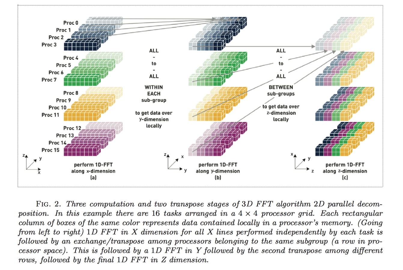
From D. Pekurovsky SIAM J. Sci. Comput., 34(4), C192–C209

N^2

N^2

Pencil decomposition

in a nutshell

rfft(u, axis=2)

Transform

fft(u, axis=0)

Transform

fft(u, axis=1)

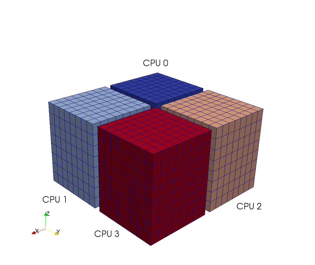
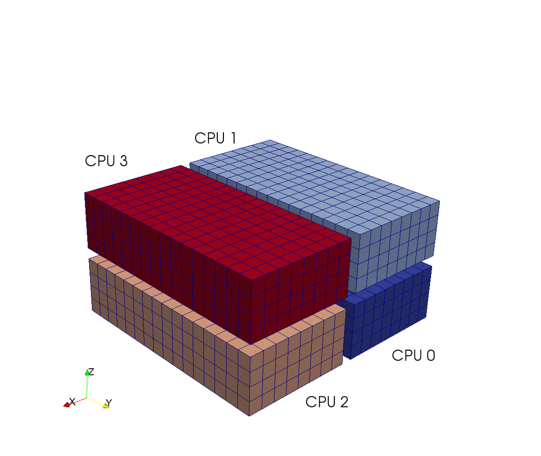
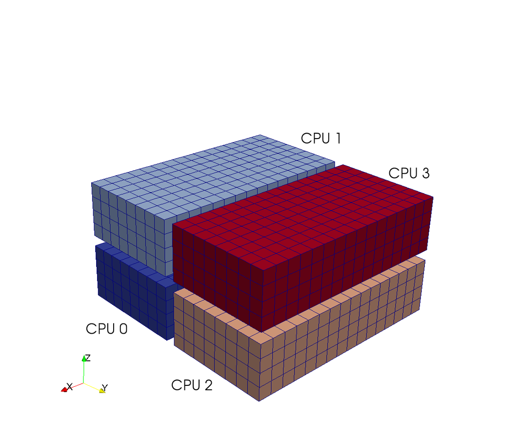
7 operations

FFT z-dir
transpose
communicate
FFT y-dir
transpose
communicate
FFT x-dir

7 lines of code!

Pencil decomposition

Implementation

rfft(u, axis=2)

Transform

fft(u, axis=1)

Transform

fft(u, axis=0)

P1 = 2                         # Parameter - Choose number of procs along x-direction
P2 = num_processes / P1        # Could use MPI.Compute_dims(num_processes, 2) to get optimal P1/P2
N1 = N / P1
N2 = N / P2
rank = comm.Get_rank()
comm0 = comm.Split(rank/P1)    # Two communicators. First one to communicate in Y-Z plan
comm1 = comm.Split(rank%P1)    # This one to communicate in X-Y plane

# Work arrays
Uc_hat_y  = numpy.zeros((N2, N, N1/2), complex)
Uc_hat_z  = numpy.zeros((N1, N2, N/2+1), complex)
Uc_hat_x  = numpy.zeros((N, N2, N1/2), complex)
Uc_hat_x2 = numpy.zeros((N, N2, N1/2), complex)
def rfftn_mpi_pencil(u, fu):
    """Pencil 3D FFT"""
    Uc_hat_z[:] = numpy.fft.rfft(u, axis=2)
    Uc_hat_x[:] = numpy.rollaxis(Uc_hat_z[:,:,:-1].reshape((N1, N2, P1, N1/2)), 2).reshape((N, N2, N1/2))
    comm0.Alltoall([Uc_hat_x, MPI.F_DOUBLE_COMPLEX], [Uc_hat_x2, MPI.F_DOUBLE_COMPLEX])
    Uc_hat_x[:] = numpy.fft.fft(Uc_hat_x2, axis=0)        
    comm1.Alltoall([Uc_hat_x, MPI.F_DOUBLE_COMPLEX], [Uc_hat_x2, MPI.F_DOUBLE_COMPLEX])  
    Uc_hat_y[:] = numpy.rollaxis(Uc_hat_x.reshape((P2, N2, N2, N1/2)), 1).reshape((N2, N, N1/2))
    fu[:] = numpy.fft.fft(Uc_hat_y, axis=1)
    return fu

# Declare variable distributed as pencil
U = numpy.random.random((N1, N2, N))
U_hat = numpy.zeros((N2, N, N1/2), complex) # This is the transform

# Perform transform
U_hat = rfftn_mpi_pencil(U, U_hat)

Done with the FFTs, how about the rest of the code?

Local Numpy ufuncs responsible for most remaining cost

# Preallocated distributed arrays. Create array of wavenumbers
K  = array(meshgrid(kx, ky, kz, indexing='ij'), dtype=float)
K2 = sum(K*K, 0, dtype=float) # Wavenumber magnitude
dU = zeros((3, N[0], Np[1], Nf), dtype=complex) # Rhs array
    
# Subtract contribution from diffusion to rhs array
dU -= nu*K2*U_hat

Besides FFT the major computational cost is computing the right hand side using element-wise numpy ufuncs (multiplications, subtractions over the entire mesh)

Very compact code

Explicit solver

Parallell scaling

Shaheen Blue Gene P supercomputer at KAUST Supercomputing Laboratory

Testing with a transient Taylor Green flow

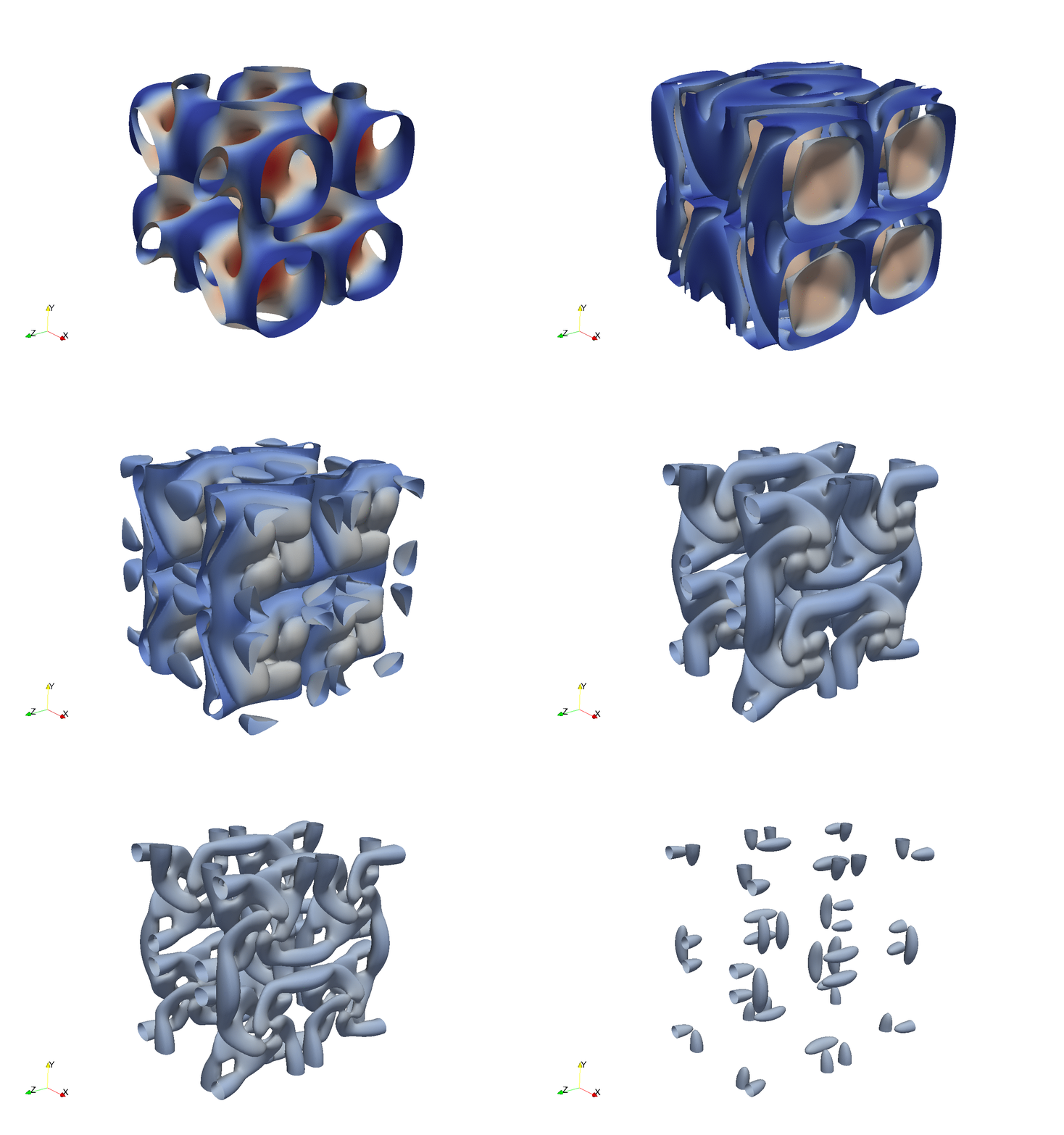
Enstrophy colored by pressure

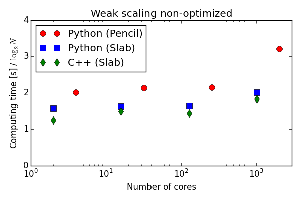
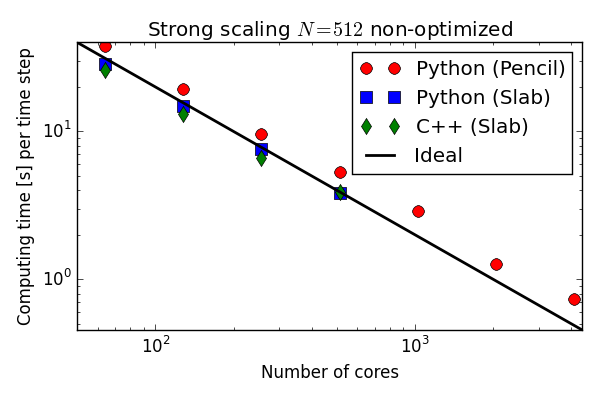
The solver has been verified to be implemented correctly, but how does the pure numpy/mpi4py/pyfftw perform?

Parallell scaling

Shaheen Blue Gene P supercomputer at KAUST Supercomputing Laboratory

Testing the 100 lines of pure Python code

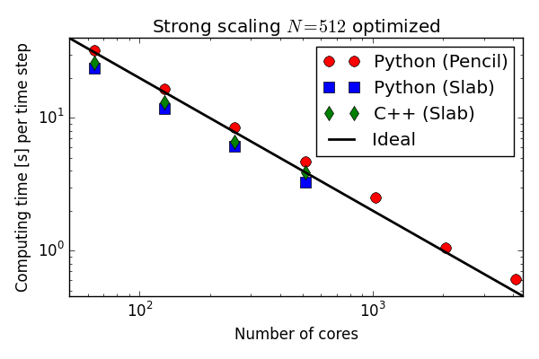
C++(slab) 20-30 % faster than Python (slab)

Good strong scaling

mesh =

2048^3

2048^3

512^3

512^3

Why slower than C++?

Actually, the numpy ufuncs used to compute rhs are the main reason

Numpy ufuncs not always great

def cross(a, b, c):
    """Regular c = a x b, with vector component in axis 0."""
    #c = numpy.cross(a, b, axis=0) # Alternative
    c[0] = a[1]*b[2]-a[2]*b[1]
    c[1] = a[2]*b[0]-a[0]*b[2]
    c[2] = a[0]*b[1]-a[1]*b[0]
    return c

N = 200
U = zeros((3, N, N, N))
W = zeros((3, N, N, N))
F = zeros((3, N, N, N))
F = cross(U, W, F)

Consider the cross product (required for rhs):

Too many ufuncs (multiplications, subtractions) are being called and too many temp arrays are created

Commented out regular numpy.cross is also using ufuncs and is about the same speed

Getting rid of some temp arrays helps

def cross(a, b, c):
    """Regular c = a x b, with vector component in axis 0."""
    c[0]  = a[1]*b[2]
    c[0] -= a[2]*b[1]
    c[1]  = a[2]*b[0]
    c[1] -= a[0]*b[2]
    c[2]  = a[0]*b[1]
    c[2] -= a[1]*b[0]    
    return c

Approximately 30% faster (for N=200),

but still too many ufuncs being called. Too many loops over the large 4D arrays a, b, c

Only viable solution

is to hardcode the cross product into one single loop

@jit(float[:,:,:,:](float[:,:,:,:], float[:,:,:,:], float[:,:,:,:]), nopython=True)
def cross(a, b, c):
    for i in xrange(a.shape[1]):
        for j in xrange(a.shape[2]):
            for k in xrange(a.shape[3]):
                a0 = a[0,i,j,k]
                a1 = a[1,i,j,k]
                a2 = a[2,i,j,k]
                b0 = b[0,i,j,k]
                b1 = b[1,i,j,k]
                b2 = b[2,i,j,k]
                c[0,i,j,k] = a1*b2 - a2*b1
                c[1,i,j,k] = a2*b0 - a0*b2
                c[2,i,j,k] = a0*b1 - a1*b0
    return c

Cython, Numba or Weave will all do the trick

Numba and Cython perform approximately the same

and as fast as C++!

Approximately 5 times faster than original

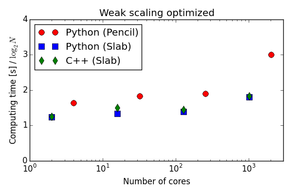
Solver optimized with Cython

More than matches C++ on the Blue Gene P!

(Numba you say? You try to install Numba on a Blue Gene)

How about Shaheen II?

Scaling tests on Shaheen II from Monday 2/5!

64^3

64^3

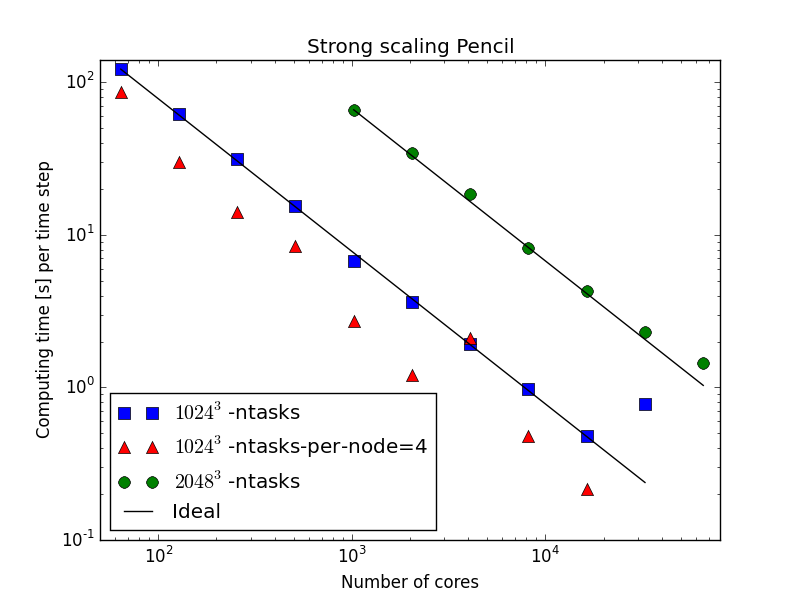
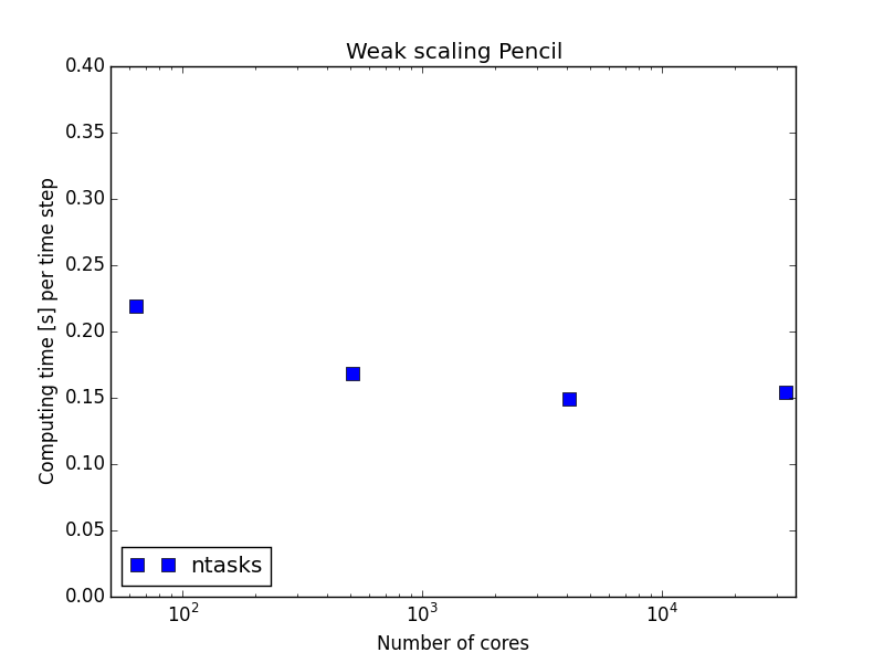
mesh size = per task

65536 tasks!

ntasks - Using just ntasks in sbatch script

ntasks-per-node specifies tasks per node

Scaling tests on Shaheen II from Monday 2/5!

64^3

64^3

mesh size = per task

65536 tasks!

mesh =

per task

Word of warning

2048 nodes, or 65536 tasks, take about 13 minutes to load Python and get started

Should have been using larger mesh

0.5 \cdot 64^3

0.5 \cdot 64^3

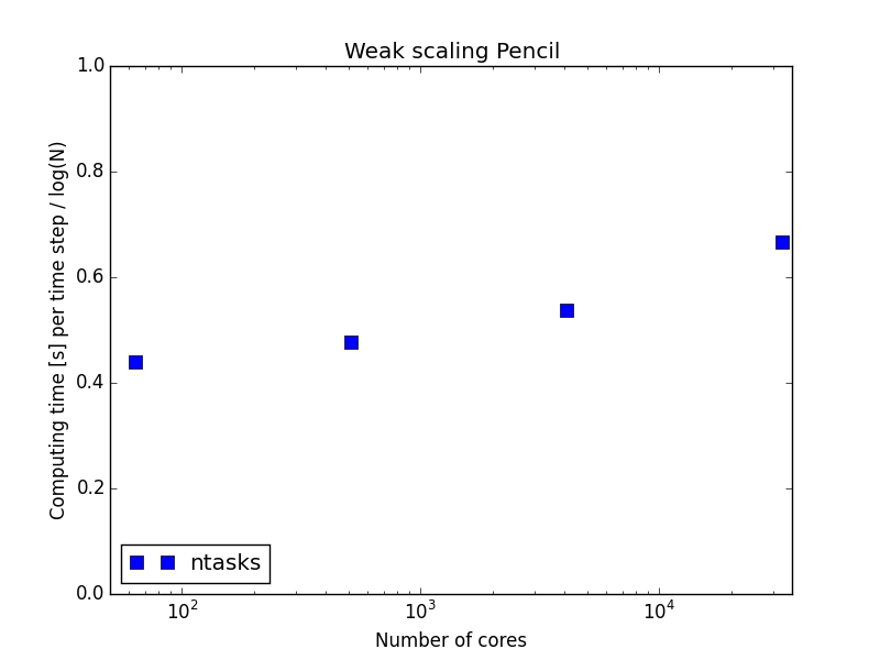
Slab results

2 \cdot 128^3

2 \cdot 128^3

mesh size = per task

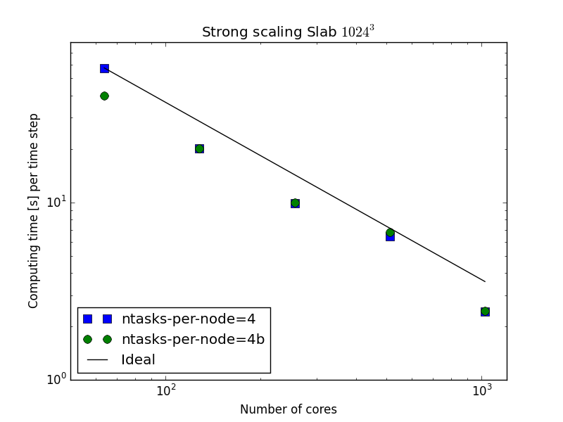
Mesh a bit too big per cpu

Would like to try smaller next time:-)

Very good scaling, but the ntasks-per-node issue

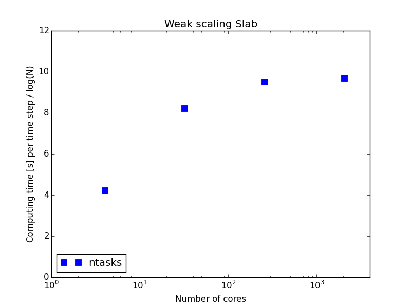
Summary

A pure Python DNS solver for turbulent flows can be created from scratch with less than 100 lines of Python code!
This code can run on thousands of processors with billions of unknowns and almost as fast (30-40% slower) as pure C++
With a few routines moved to Cython, the Python based solver matches the performance of C++
Interested in helping out? Think you can do better?
- https://github.com/spectralDNS
- Currently DNS solvers for incompressible/variable density Navier Stokes and Magneto Hydro Dynamics Isotropic (triply periodic) and channel flows

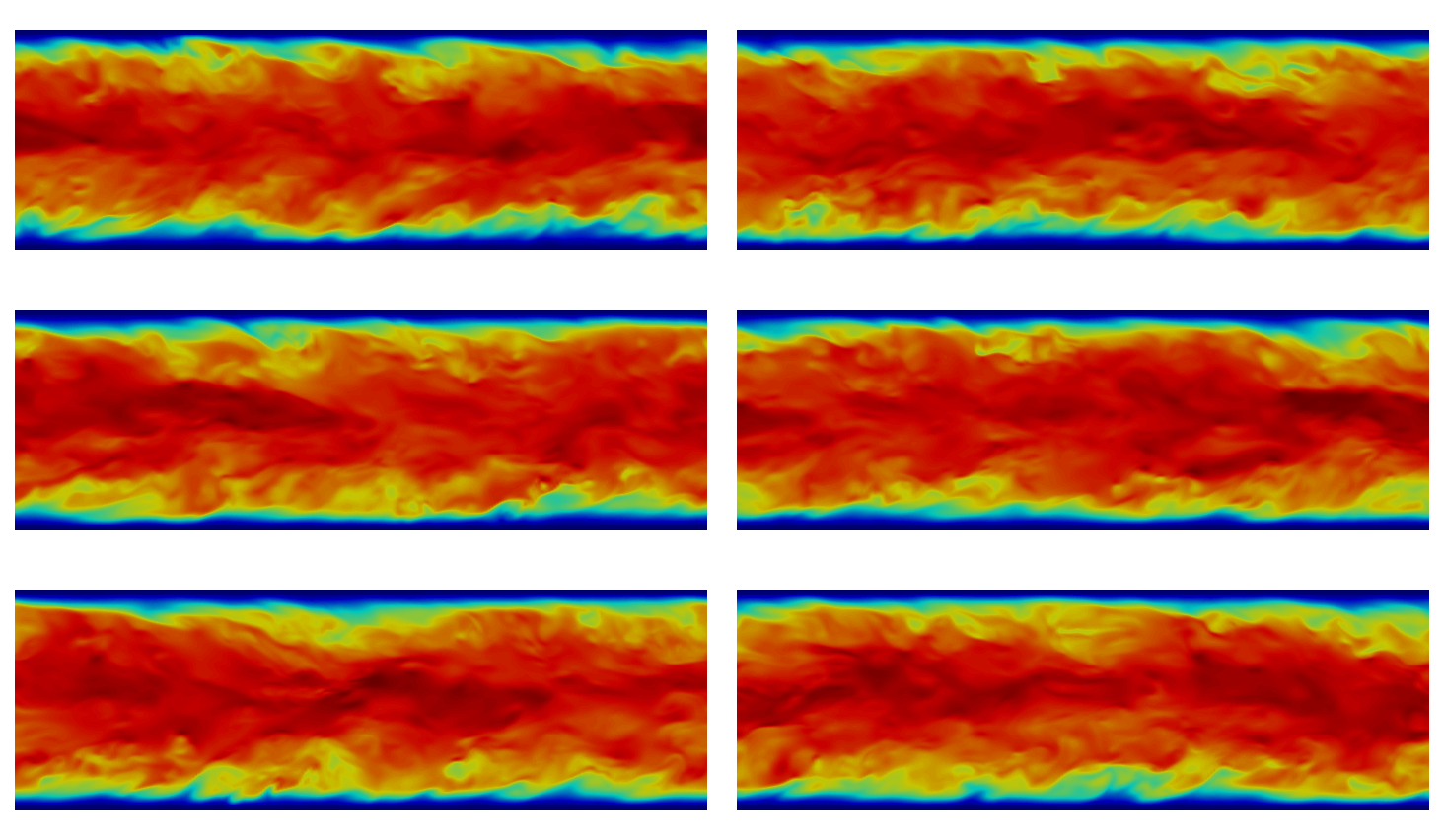
Turbulent Channel solver

Currently running with using 512 CPUs on ShaheenII

512^3

512^3

Re_{\tau} = 590

Re_{\tau} = 590

Thanks also to Hans Petter Langtangen at UiO/Simula

and David Ketcheson and Bilel Hadri at KAUST

Thank you for your attention!

Massively parallel at KAUST

By Mikael Mortensen

Massively parallel at KAUST

Massively parallel implementation in Python of a pseudo-spectral DNS code for turbulent flows

Direct Numerical Simulations of turbulence are performed with low-level Fortran or C

Is it possible to write a competitive, state of the art turbulence solver in Python?

Turbulence is governed by the Navier Stokes equations

Navier Stokes in spectral space

Implementation

mpi4py

3D FFT with MPI

3D FFT with MPI

What does it really take?

3D FFT with MPI

Pencil decomposition

Pencil decomposition

Pencil decomposition

Done with the FFTs, how about the rest of the code?

Local Numpy ufuncs responsible for most remaining cost

Parallell scaling

Parallell scaling

Why slower than C++?

Numpy ufuncs not always great

Getting rid of some temp arrays helps

Only viable solution

Solver optimized with Cython

How about Shaheen II?

Scaling tests on Shaheen II from Monday 2/5!

Scaling tests on Shaheen II from Monday 2/5!

Slab results

Summary

Turbulent Channel solver

Thank you for your attention!

Massively parallel at KAUST

More from Mikael Mortensen