CS6015: Linear Algebra and Random Processes
Lecture 12: Projecting a vector onto another vector, Projecting a vector on to a subspace, Linear Regression (Least Squares)
Learning Objectives
How do you project a vector onto another vector?
(for today's lecture)
How do you project a vector onto a subspace?
What is "linear regression" or "least squares" method?
Projecting a vector on another vector
\mathbf{a}
\mathbf{b}
\mathbf{p}
\mathbf{e} = \mathbf{b} - \mathbf{p}
=\hat{x}\mathbf{a}
\mathbf{a}^\top\mathbf{e} = 0
(orthogonal vectors)
\mathbf{a}^\top(\mathbf{b} - \mathbf{p}) = 0
\mathbf{a}^\top(\mathbf{b} - \hat{x}\mathbf{a}) = 0
\mathbf{a}^\top\mathbf{b} - \hat{x}\mathbf{a}^\top\mathbf{a} = 0
\hat{x} = \frac{\mathbf{a}^\top\mathbf{b}}{\mathbf{a}^\top\mathbf{a}}
\mathbf{p} = \hat{x}\mathbf{a} = \mathbf{a}\frac{\mathbf{a}^\top\mathbf{b}}{\mathbf{a}^\top\mathbf{a}}
\therefore \mathbf{p} = \frac{\mathbf{a}\mathbf{a}^\top}{\mathbf{a}^\top\mathbf{a}} \mathbf{b}
\begin{bmatrix}
a_1\\
a_2\\
\cdots\\
a_n
\end{bmatrix}
\begin{bmatrix}
a_1&
a_2&
\cdots&
a_n
\end{bmatrix}
\mathbf{a}
\mathbf{a}^\top
n\times1
1\times n
\mathbf{a}\mathbf{a}^\top~is~a~n\times n~matrix
\therefore \mathbf{p} = P\mathbf{b}
The Projection matrix
\mathbf{a}
\mathbf{b}
\mathbf{p}
\mathbf{e} = \mathbf{b} - \mathbf{p}
=x\mathbf{a}
P = \frac{1}{\mathbf{a}^\top\mathbf{a}} \mathbf{a}\mathbf{a}^\top
P^\top = P
P^2 =
\frac{1}{\mathbf{a}^\top\mathbf{a}} \mathbf{a}\mathbf{a}^\top \frac{1}{\mathbf{a}^\top\mathbf{a}} \mathbf{a}\mathbf{a}^\top
=(\frac{1}{\mathbf{a}^\top\mathbf{a}})^2 \mathbf{a}\mathbf{a}^\top \mathbf{a}\mathbf{a}^\top
= \frac{1}{\mathbf{a}^\top\mathbf{a}} \mathbf{a}\mathbf{a}^\top
= P
(multiplying any vector by \( P \) will project that vector onto \(\mathbf{a}\))
\mathcal{C}(P) =
a line - all multiples of \(\mathbf{a}\)
Recap: Goal: Project onto a subspace
\begin{bmatrix}
a_{11}&~&a_{12}&~&a_{13}&~&a_{14}&~&a_{15}&\cdots&a_{1n}\\
72&~&84&~&175&~&\cdots&~&\cdots&\cdots&78\\
72&~&84&~&175&~&\cdots&~&\cdots&\cdots&78\\
\cdots&~&\cdots&~&\cdots&~&\cdots&~&\cdots&\cdots&\cdots\\
\cdots&~&\cdots&~&\cdots&~&\cdots&~&\cdots&\cdots&\cdots\\
a_{m1}&~&a_{m2}&~&a_{m3}&~&a_{m4}&~&a_{m5}&\cdots&a_{mn}\\
\end{bmatrix}
=\begin{bmatrix}
b_{1}\\
110\\
120\\
\cdots\\
\cdots\\
b_{m}\\
\end{bmatrix}
\begin{bmatrix}
x_{1}\\
x_{2}\\
x_{3}\\
\cdots\\
\cdots\\
x_{n}\\
\end{bmatrix}
A
\mathbf{b}
\mathbf{b}
column space of A
\mathbf{p}
\begin{bmatrix}
p_{1}\\
115\\
115\\
\cdots\\
\cdots\\
p_{m}\\
\end{bmatrix}
\mathbf{p}
"Project" \(\mathbf{b} \) into the column space of \(A\)
Solve \( A\mathbf{\hat{x}} = \mathbf{p}\)
\( \mathbf{\hat{x}}\) is the best possible approximation
\(\mathbf{b} \) is not in the column space of \(A\)
Hence no solution to \(A\mathbf{x} = \mathbf{b} \)
Projecting onto a subspace
Let~Basis(\mathcal{C}(A)) = \mathbf{a}_1, \mathbf{a}_2
\mathbf{b}
column space of A
\mathbf{p}
How would you express \(\mathbf{p}\)?
p = \mathbf{a}_1\hat{x_1}+\mathbf{a}_2\hat{x_2}
(it will be some linear combination of the columns of A)
Let~A = \begin{bmatrix}
\uparrow&\uparrow\\
\mathbf{a}_1&\mathbf{a}_2\\
\downarrow&\downarrow
\end{bmatrix}
Our goal: Solve \(A\mathbf{\hat{x}} = \mathbf{p}\)
(we are looking for a similar neat formula for )
\mathbf{\hat{x}}
\mathbf{a}_1
\mathbf{a}_2
\mathbf{a}
\mathbf{b}
\mathbf{p}
\mathbf{e} = \mathbf{b} - \mathbf{p}
=\hat{x}\mathbf{a}
\hat{x} = \frac{\mathbf{a}^\top\mathbf{b}}{\mathbf{a}^\top\mathbf{a}}
Recap
Projecting onto a subspace
\mathbf{e} = \mathbf{b} - \mathbf{p}
\mathbf{b}
column space of A
\mathbf{p}
\mathbf{a}_1
\mathbf{a}_2
\mathbf{e} = \mathbf{b} - \mathbf{p}
\mathbf{e} = \mathbf{b} - A\mathbf{\hat{x}}
\mathbf{a}_1^\top(\mathbf{b} - A\mathbf{\hat{x}}) = 0
\mathbf{a}_2^\top(\mathbf{b} - A\mathbf{\hat{x}}) = 0
\begin{bmatrix}
\leftarrow&\mathbf{a}_1^\top&\rightarrow\\
\leftarrow&\mathbf{a}_2^\top&\rightarrow\\
\end{bmatrix}(\mathbf{b} - A\mathbf{\hat{x}}) = \begin{bmatrix}0\\0\end{bmatrix}
A^\top(\mathbf{b} - A\mathbf{\hat{x}}) = \mathbf{0}
(\mathbf{b} - A\mathbf{\hat{x}}) \in \mathcal{N}(A^\top)
(\mathbf{b} - A\mathbf{\hat{x}}) \perp \mathcal{C}(A)
Projecting onto a subspace
\mathbf{b}
column space of A
\mathbf{p}
\mathbf{a}_1
\mathbf{a}_2
\mathbf{e} = \mathbf{b} - \mathbf{p}
\mathbf{a}
\mathbf{b}
\mathbf{p}
\mathbf{e} = \mathbf{b} - \mathbf{p}
=\hat{x}\mathbf{a}
\mathbf{a}^\top(\mathbf{b} - \hat{x}\mathbf{a}) = 0
\hat{x} = \frac{\mathbf{a}^\top\mathbf{b}}{\mathbf{a}^\top\mathbf{a}}
\mathbf{p} = \frac{\mathbf{a}\mathbf{a}^\top}{\mathbf{a}^\top\mathbf{a}} \mathbf{b}
Recap
A^\top(\mathbf{b} - A\mathbf{\hat{x}}) = \mathbf{0}
A^\top A\mathbf{\hat{x}} = A^\top\mathbf{b}
\mathbf{\hat{x}} = (A^\top A)^{-1}A^\top\mathbf{b}
\mathbf{p} = A\mathbf{\hat{x}}
\mathbf{p} = A(A^\top A)^{-1}A^\top\mathbf{b}
P = A(A^\top A)^{-1}A^\top
How do I know this inverse exists?
The invertibility of \(A^\top A\)
Theorem: If \(A\) has \(n\) independent columns then \(A^\top A\) is invertible
Proof: HW4
We can rely on this result because we have assumed \(A\) contains independent columns
What if that is not the case?
Just do GE and retain independent columns
(we anyways set the dependent variables to 0 while finding x particular)
(There is another alternative which you will see soon)
Properties of \(P\)
P = A(A^\top A)^{-1}A^\top
P^\top = P
P^2 = A(A^\top A)^{-1}A^\top
A(A^\top A)^{-1}A^\top
P^2 = A(A^\top A)^{-1}A^\top = P
HW4: What if \(A\) is a full rank square matrix?
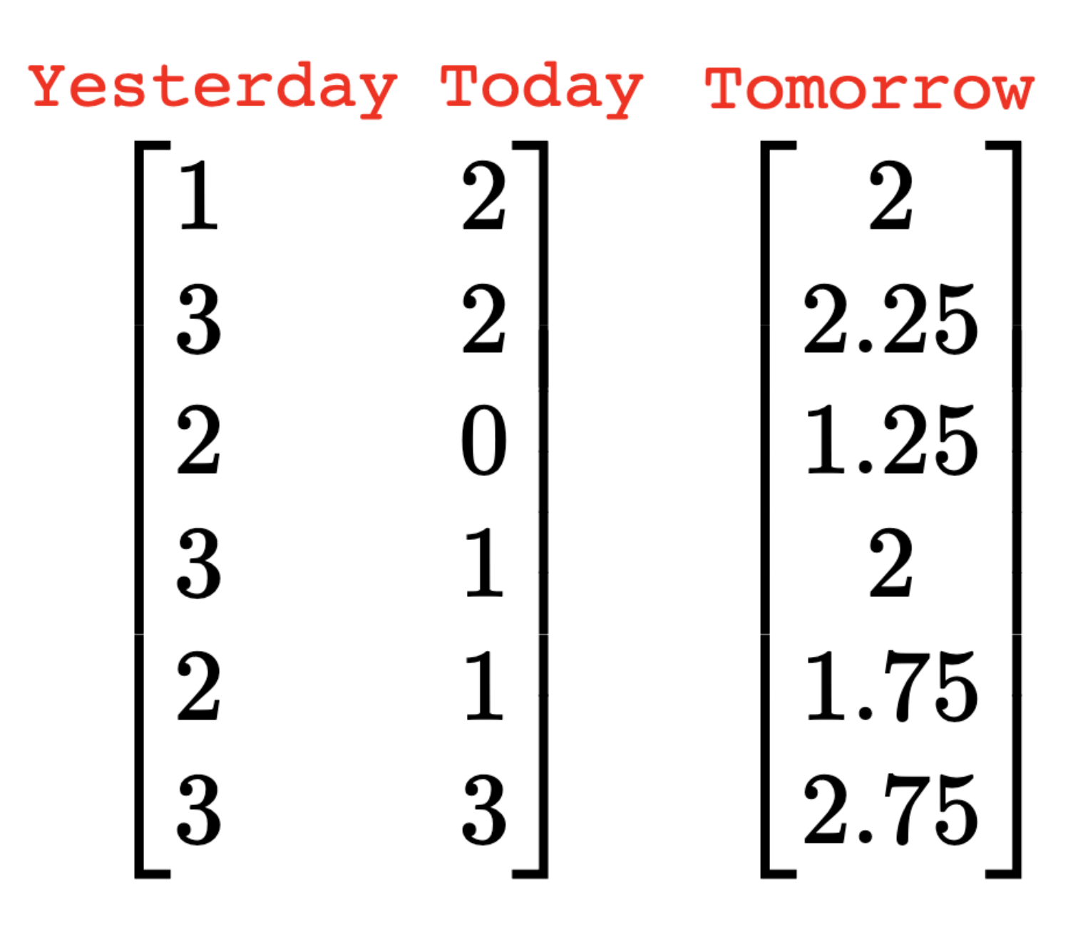
Back to our ML example
Yesterday
How many COVID19 cases would be there tomorrow?
Loc. 1
Loc. 2
Loc. 3
Loc. m
Tomorrow
\begin{bmatrix}
a_{11}&~&a_{12}\\
a_{21}&~&a_{22}\\
a_{31}&~&a_{32}\\
\cdots&~&\cdots\\
\cdots&~&\cdots\\
a_{m1}&~&a_{m2}\\
\end{bmatrix}
\begin{bmatrix}
b_{1}\\
b_{2}\\
b_{3}\\
\cdots\\
\cdots\\
b_{m}\\
\end{bmatrix}
You know that some relation exists between '# of cases' and the 2 variables
But you don't know what \( f \) is!
b_{1} = f(a_{11}, a_{12})
We will just assume that it is linear
(a toy example)
Today
(In practice, there would be many more variables but for simplicity and ease of visualisation we consider only 2 variables)
\begin{bmatrix}
x_{1}\\
x_{2}
\end{bmatrix}
=
b = x_1*a_{yesterday} + x_2*a_{today}
Back to our ML example
Yesterday
Tomorrow
\begin{bmatrix}
1&~&2\\
3&~&2\\
2&~&0\\
3&~&1\\
2&~&1\\
3&~&3\\
\end{bmatrix}
(a toy example)
Today
\begin{bmatrix}
x_{1}\\
x_{2}
\end{bmatrix}
=
\begin{bmatrix}
2\\
2.25\\
1.25\\
2\\
1.75\\
2.75\\
\end{bmatrix}
Loc. 1
Loc. 2
Loc. 3
Loc. 6
b = x_1*a_{yesterday} + x_2*a_{today}
Does the above system of equations have a solution?
Practice Problem: Perform Gaussian Elimination and check whether the above system of equations has a solution
It does not but still verify it!
So what do we do?
\(\mathbf{b}\) is not in the column space of \(A\)
\begin{bmatrix}
1&~&2\\
3&~&2\\
2&~&0\\
3&~&1\\
2&~&1\\
3&~&3\\
\end{bmatrix}
\begin{bmatrix}
x_{1}\\
x_{2}
\end{bmatrix}
=
A
\mathbf{x}
\mathbf{b}
Find its projection \(\mathbf{p}\)
Solve \(A\mathbf{\hat{x}} = \mathbf{p}\)
Recap
A^\top A\mathbf{\hat{x}} = A^\top\mathbf{b}
\mathbf{\hat{x}} = (A^\top A)^{-1}A^\top\mathbf{b}
\begin{bmatrix}
2\\
2.25\\
1.25\\
2\\
1.75\\
2.75\\
\end{bmatrix}
column space of A
\mathbf{a}_1\in \mathbb{R}^6
\mathbf{a}_2\in \mathbb{R}^6
\( \mathcal{C}(A)\) is a 2d plane in a 6 dimensional space
\mathbf{b}\in \mathbb{R}^6
\mathbf{p}
Finding \( \hat{\mathbf{x}}\)
\begin{bmatrix}
1&~&2\\
3&~&2\\
2&~&0\\
3&~&1\\
2&~&1\\
3&~&3\\
\end{bmatrix}
\begin{bmatrix}
x_{1}\\
x_{2}
\end{bmatrix}
=
A^\top
A
\mathbf{\hat{x}}
Recap
A^\top A\mathbf{\hat{x}} = A^\top\mathbf{b}
\begin{bmatrix}
1&3&2&3&2&3\\
2&2&0&1&1&3
\end{bmatrix}
A^\top
\begin{bmatrix}
1&3&2&3&2&3\\
2&2&0&1&1&3
\end{bmatrix}
\mathbf{b}
\begin{bmatrix}
36&22\\
22&19
\end{bmatrix}
\begin{bmatrix}
x_{1}\\
x_{2}
\end{bmatrix}
\mathbf{\hat{x}}
=\begin{bmatrix}
29\\
20.5
\end{bmatrix}
\begin{bmatrix}
2\\
2.25\\
1.25\\
2\\
1.75\\
2.75\\
\end{bmatrix}
x_{1}=0.5\\
x_{2}=0.5
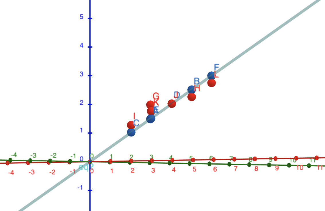
The two geometric views
b = 0.5*a_{yesterday} + 0.5*a_{today}
b
a_{yesterday}
a_{today}
column space of A
\mathbf{a}_1\in \mathbb{R}^6
\mathbf{a}_2\in \mathbb{R}^6
\mathbf{b}\in \mathbb{R}^6
\mathbf{p}
\(b\) is a function of the inputs
We have assumed this function to be linear
What is the geometric interpretation?
(switch to geogebra)
One method, many names
We are "fitting a line/plane"
We are doing "linear regression"
We are finding the "least squares" solution
(How?)
\min_{\mathbf{p}} ||\mathbf{b} - \mathbf{p}||_2^2
\min_{\mathbf{\hat{x}}} ||\mathbf{b} - A\mathbf{\hat{x}}||_2^2
\begin{bmatrix}
b_1\\
b_2\\
b_3\\
\cdots\\
b_m\\
\end{bmatrix}
\begin{bmatrix}
p_1\\
p_2\\
p_3\\
\cdots\\
p_m\\
\end{bmatrix}
\begin{bmatrix}
b_1-p_1\\
b_2-p_2\\
b_3-p_3\\
\cdots\\
b_m-p_m\\
\end{bmatrix}
\mathbf{b}-\mathbf{p}
\min_{\mathbf{\hat{x}}} (\mathbf{b} - A\mathbf{\hat{x}})^\top(\mathbf{b} - A\mathbf{\hat{x}})
\min_{\mathbf{\hat{x}}} (\mathbf{b}^\top - \mathbf{\hat{x}}^\top A^\top)(\mathbf{b} - A\mathbf{\hat{x}})
\min_{\mathbf{\hat{x}}} (\mathbf{b}^\top - \mathbf{\hat{x}}^\top A^\top)(\mathbf{b} - A\mathbf{\hat{x}})
\min_{\mathbf{\hat{x}}} (\mathbf{b}^\top\mathbf{b} - \mathbf{\hat{x}}^\top A^\top\mathbf{b} - \mathbf{b}^\top A\mathbf{\hat{x}} + \mathbf{x}^\top A^\top A\mathbf{\hat{x}})
Take derivative w.r.t \( \mathbf{\hat{x}} \) and set to 0
2A^\top\mathbf{b} - 2A^\top A\mathbf{\hat{x}} = 0
\implies A^\top A\mathbf{\hat{x}} = A^\top\mathbf{b}
Learning Objectives
(achieved)
How do you project a vector onto another vector?
How do you project a vector onto a subspace?
What is "linear regression" or "least squares" method?
CS6015: Lecture 12
By Mitesh Khapra
CS6015: Lecture 12
Lecture 12: Projecting a vector onto another vector, Projecting a vector on to a subspace, Solving Ax=b when no solution exists


