CS6015: Linear Algebra and Random Processes
Lecture 18: Diagonalisation (Eigenvalue Decomposition) of a matrix, Computing powers of A
Learning Objectives
What is eigenvalue decomposition?
What do we mean by diagonalisation of a matrix?
or
Why do we care about diagonalisation?
The Eigenstory
real
imaginary
distinct
repeating
\(A^\top\)
\(A^{-1}\)
\(AB\)
\(A^\top A\)
(basis)
powers of A
PCA
optimisation
diagonalisation
\(A+B\)
\(U\)
\(R\)
\(A^2\)
\(A + kI\)
How to compute eigenvalues?
What are the possible values?
What are the eigenvalues of some special matrices ?
What is the relation between the eigenvalues of related matrices?
What do eigen values reveal about a matrix?
What are some applications in which eigenvalues play an important role?
Identity
Projection
Reflection
Markov
Rotation
Singular
Orthogonal
Rank one
Symmetric
Permutation
det(A - \lambda I) = 0
trace
determinant
invertibility
rank
nullspace
columnspace
(positive semidefinite matrices)
positive pivots
(independent eigenvectors)
(orthogonal eigenvectors)
... ...
(symmetric)
(where are we?)
(characteristic equation)
(desirable)
HW5
distinct values
independent eigenvectors
\(\implies\)
steady state
(Markov matrices)
eigenvalues
The bigger picture
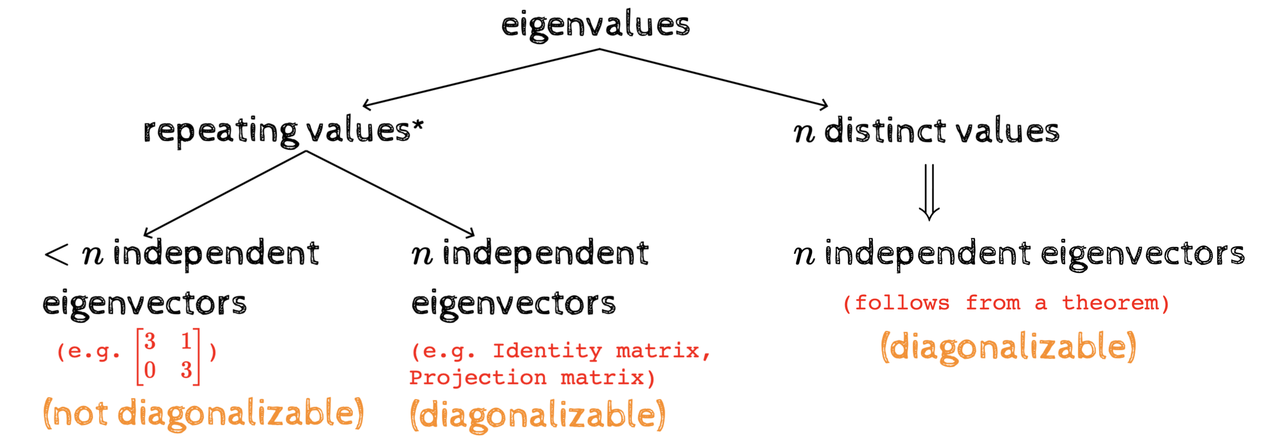
\(n\) distinct values
\(\implies\)
\(n\) independent eigenvectors
(follows from a theorem)
repeating values*
* more than 1 value can repeat - e.g. in a projection matrix both the eigenvalues 1 and 0 may repeat
\(n\) independent eigenvectors
\(<n\) independent eigenvectors
(e.g. Identity matrix, Projection matrix)
(diagonalizable)
(diagonalizable)
(not diagonalizable)
\begin{bmatrix}
3&1\\
0&3
\end{bmatrix}
(e.g. )
The bigger picture
* more than 1 value can repeat - e.g. in a projection matrix both the eigenvalues 1 and 0 may repeat
(questions)
What do we mean by saying that a matrix is diagonalizable?
Why do we care about diagonalizability?
What is the condition under which we will have \(n\) independent vectors even with repeating eigenvalues?
The bigger picture
* more than 1 value can repeat - e.g. in a projection matrix both the eigenvalues 1 and 0 may repeat
As usual we will focus on the good case first!
The good case: n independent eigenvectors
Theorem (HW5): If eigenvectors \(s_1, \dots, s_n\) correspond to different eigenvalues \(\lambda_1, \dots, \lambda_n\) , then those eigenvectors are linearly independent
Construct a matrix \(S\) whose columns are these \(n\) independent eigenvectors
\begin{bmatrix}
\uparrow&\uparrow&\dots&\uparrow\\
s_1&s_2&\dots&s_n\\
\downarrow&\downarrow&\dots&\downarrow\\
\end{bmatrix}
S
A
=\begin{bmatrix}
\uparrow&\uparrow&\dots&\uparrow\\
As_1&As_2&\dots&As_n\\
\downarrow&\downarrow&\dots&\downarrow\\
\end{bmatrix}
=\begin{bmatrix}
\uparrow&\uparrow&\dots&\uparrow\\
\lambda_1s_1&\lambda_2s_2&\dots&\lambda_ns_n\\
\downarrow&\downarrow&\dots&\downarrow\\
\end{bmatrix}
=\begin{bmatrix}
\uparrow&\uparrow&\dots&\uparrow\\
s_1&s_2&\dots&s_n\\
\downarrow&\downarrow&\dots&\downarrow\\
\end{bmatrix}
\begin{bmatrix}
\lambda_1&0&\dots&0\\
0&\lambda_2&\dots&0\\
\dots&\dots&\dots&\lambda_n\\
\end{bmatrix}
AS = S\Lambda
The good case: n independent eigenvectors
AS = S\Lambda
A = S\Lambda S^{-1}
S^{-1}AS = \Lambda
\(S\) is invertible as it is a square matrix with independent columns
(diagonalisation)
(eigenvalue decomposition)
Why do we care about diagonalisation?
Let's look at some applications
Powers of \(A\)
A\mathbf{x} = \lambda \mathbf{x}
A^2\mathbf{x} = AA\mathbf{x} = A\lambda \mathbf{x} = \lambda A\mathbf{x} = \lambda^2 \mathbf{x}
A^3\mathbf{x} = AA^2\mathbf{x} = A\lambda^2 \mathbf{x} = \lambda^2 A\mathbf{x} = \lambda^3 \mathbf{x}
A^n\mathbf{x} = \lambda^n \mathbf{x}
Powers of \(A\) have the same eigenvectors as \(A\) with the eigenvalues raised to the appropriate power
Powers of \(A\)
Powers of \(A\) have the same eigenvectors as \(A\) with the eigenvalues raised to the appropriate power
(the diagonalized view)
A = S\Lambda S^{-1}
A^2 = S\Lambda S^{-1}S\Lambda S^{-1}
=S\Lambda\Lambda S^{-1}
=S\Lambda^2 S^{-1}
A^3 = AA^2 = S\Lambda S^{-1}S\Lambda^2 S^{-1}
=S\Lambda^3 S^{-1}
A^n=S\Lambda^n S^{-1}
Powers of \(A\)
Imagine a particle in 2d space
(why do we care?)
\mathbf{v}_0=\begin{bmatrix}
2\\1
\end{bmatrix}
Suppose the particle moves to a new location every second
The displacement is given by a matrix
\begin{bmatrix}
1&0.5\\
0.5&1\\
\end{bmatrix}
Where would the particle be after 24 hours (86400 seconds)?
Powers of \(A\)
1 sec:
(why do we care?)
A\mathbf{v}_0
Where would the particle be after 24 hours (86400 seconds)?
2 sec:
AA\mathbf{v}_0=A^2\mathbf{v}_0
3 sec:
A^3\mathbf{v}_0
... ...
... ...
86400 sec:
A^{86400}\mathbf{v}_0
(very expensive computation)
But what if we use the EVD of A?
\mathbf{v}_0=\begin{bmatrix}
2\\1
\end{bmatrix}
Powers of \(A\)
(use EVD of A \(\equiv\) change of basis)
k seconds:
A^{k}\mathbf{v}_0
S\Lambda^{k}S^{-1}\mathbf{v}_0
\overbrace{~~~~~~~~~~~~~~}
\underbrace{~~~~~~~~~~~}
Eigenbasis:
Translating from std. basis to eigenbasis
The basis formed by the eigenvectors of \(A\)
The transformation becomes very simple in this basis
Translate back to the standard basis
(A becomes diagonal in this basis)
\mathbf{v}_0=\begin{bmatrix}
2\\1
\end{bmatrix}
Powers of \(A\)
(computational efficiency)
[\mathbf{v}]_S
S^{-1}
[A^k\mathbf{v}]_S
\Lambda^k
O(n^2)
A^{k}\mathbf{v} = S\Lambda^{k}S^{-1}\mathbf{v}
S
O(n^2)
O(nk)
O(kn^3)
O(n^2 + nk + n^2)
+ the cost of computing EVs
EVD/Diagonalization/Eigenbasis is useful when the same matrix \(A\) operates on many vectors repeatedly (i.e., if we want to apply \(A^n\) to many vectors)
(this one time cost is then justified in the long run)
\mathbf{v}
A^k\mathbf{v}
A^k
O(kn^3)
The Eigenstory
real
imaginary
distinct
repeating
\(A^\top\)
\(A^{-1}\)
\(AB\)
\(A^\top A\)
(basis)
powers of A
steady state
PCA
optimisation
diagonalisation
\(A+B\)
\(U\)
\(R\)
\(A^2\)
\(A + kI\)
How to compute eigenvalues?
What are the possible values?
What are the eigenvalues of some special matrices ?
What is the relation between the eigenvalues of related matrices?
What do eigen values reveal about a matrix?
What are some applications in which eigenvalues play an important role?
Identity
Projection
Reflection
Markov
Rotation
Singular
Orthogonal
Rank one
Symmetric
Permutation
det(A - \lambda I) = 0
trace
determinant
invertibility
rank
nullspace
columnspace
(Markov matrices)
(positive semidefinite matrices)
positive pivots
(independent eigenvectors)
(orthogonal eigenvectors)
... ...
(symmetric)
(where are we?)
(characteristic equation)
(desirable)
HW5
distinct values
independent eigenvectors
\(\implies\)
Let's dig a bit deeper into our previous example
Where would the particle land?
A = \begin{bmatrix}
1&0.5\\
0.5&1\\
\end{bmatrix}
(after 100 sec.)
\mathbf{v}_0=\begin{bmatrix}
2\\1
\end{bmatrix}
A = S\Lambda S^{-1}
\Lambda = \begin{bmatrix}
1.5&0\\
0&0.5\\
\end{bmatrix}
S = \begin{bmatrix}
1&-1\\
1&1\\
\end{bmatrix}
S^{-1} = \frac{1}{2}\begin{bmatrix}
1&1\\
-1&1\\
\end{bmatrix}
(orthogonal)
A^{100}\mathbf{v}_0 = S\Lambda^{100} S^{-1}\mathbf{v}_0
=\frac{1}{2}\begin{bmatrix}
1&-1\\
1&1\\
\end{bmatrix}
\begin{bmatrix}
1.5^{100}&0\\
0&0.5^{100}\\
\end{bmatrix}
\begin{bmatrix}
1&1\\
-1&1\\
\end{bmatrix}
\begin{bmatrix}
2\\
1\\
\end{bmatrix}
\mathbf{v}_0=\begin{bmatrix}
2\\1
\end{bmatrix}
Where would the particle land?
(after 100 sec.)
\frac{1}{2}\begin{bmatrix}
1&-1\\
1&1\\
\end{bmatrix}
\begin{bmatrix}
1.5^{100}&0\\
0&0.5^{100}\\
\end{bmatrix}
\begin{bmatrix}
1&1\\
-1&1\\
\end{bmatrix}
\begin{bmatrix}
2\\
1\\
\end{bmatrix}
\approx 0
\frac{1}{2}\begin{bmatrix}
1*1.5^{100}&\approx0\\
1*1.5^{100}&\approx0\\
\end{bmatrix}
\begin{bmatrix}
1&1\\
-1&1\\
\end{bmatrix}
\begin{bmatrix}
2\\
1\\
\end{bmatrix}
\frac{1.5^{100}}{2}\begin{bmatrix}
1&0\\
1&0\\
\end{bmatrix}
\begin{bmatrix}
1&1\\
-1&1\\
\end{bmatrix}
\begin{bmatrix}
2\\
1\\
\end{bmatrix}
\frac{1.5^{100}}{2}\begin{bmatrix}
1&1\\
1&1\\
\end{bmatrix}
\begin{bmatrix}
2\\
1\\
\end{bmatrix}
\frac{1.5^{100}}{2}\begin{bmatrix}
3\\
3\\
\end{bmatrix}
=\frac{3*1.5^{100}}{2}\begin{bmatrix}
1\\
1\\
\end{bmatrix}
\mathbf{v}_0=\begin{bmatrix}
2\\1
\end{bmatrix}
\begin{bmatrix}
-1\\1
\end{bmatrix}
=k\begin{bmatrix}
1\\
1\\
\end{bmatrix}
\begin{bmatrix}
1\\1
\end{bmatrix}
A^{100}\mathbf{v}_0 =
(some multiple of the dominant eigenvector)
Where would the particle land?
(after 100 sec.)
\mathbf{v}_0=\begin{bmatrix}
2\\1
\end{bmatrix}
\begin{bmatrix}
-1\\1
\end{bmatrix}
k\begin{bmatrix}
1\\
1\\
\end{bmatrix}
\begin{bmatrix}
1\\1
\end{bmatrix}
A^{100}\mathbf{v}_0 =
(some multiple of the dominant eigenvector)

If \(\lambda_1, \lambda_2, \dots, \lambda_n\) are the eigenvalues of a matrix then \(\lambda_i\) is called the dominant eigenvalue if \(|\lambda_i| \geq |\lambda_j|~\forall j\neq i\)
The corresponding eigenvector is called the dominant eigenvector \(e_d\)
\lambda=1.5
\lambda=0.5
Observation:
\mathbf{v_0}, A\mathbf{v_0}, A^2\mathbf{v_0}, A^3\mathbf{v_0}, \dots, ke_d
Was this a coincidence?
No!
(proof on next slide)
What does this sequence approach?
\mathbf{v}_0 = c_1\mathbf{s}_1 + c_2\mathbf{s}_2 + \cdots + c_n\mathbf{s}_n
\mathbf{v_0}, A\mathbf{v_0}, A^2\mathbf{v_0}, A^3\mathbf{v_0},~to~ke_d
(n independent eigenvectors form a basis. Hence any vector can be written as their linear combination)
A^{k}\mathbf{v}_0 = c_1A^{k}\mathbf{s}_1 + c_2A^{k}\mathbf{s}_2 + \cdots + c_nA^{k}\mathbf{s}_n
A^{k}\mathbf{v}_0 = c_1\lambda_1^{k}\mathbf{s}_1 + c_2\lambda_2^{k}\mathbf{s}_2 + \cdots + c_n\lambda_n^{k}\mathbf{s}_n
(without loss of generality let lambda1 be the dominant eigenvalue)
A^{k}\mathbf{v}_0 = \lambda_1^{k}(c_1\mathbf{s}_1 + c_2(\frac{\lambda_2}{\lambda_1})^{k}\mathbf{s}_2 + \cdots + c_n(\frac{\lambda_n}{\lambda_1})^{k}\mathbf{s}_n)
As~k\rightarrow\infty~~(\frac{\lambda_i}{\lambda_1})^k \rightarrow 0
\underbrace{~~~~~~~~~~~~~~~~~~~~~~~~~~~~~~~~~~~~~~~~~~~~~~~~~~}
(hence these terms will disappear)
A^{k}\mathbf{v}_0 \rightarrow \lambda_1^{k}c_1\mathbf{s}_1
(some multiple of the dominant eigenvector)
Note that this result does holds true irrespective of the initial value \(\mathbf{v_0}\)
(as long as c1 is not 0)
What does this sequence approach?
\mathbf{v_0}, A\mathbf{v_0}, A^2\mathbf{v_0}, A^3\mathbf{v_0},~to~ke_d
This method of finding the dominant eigenvector is called Power Iteration or the Power method
The sequence approaches the dominant eigenvector of \(A\)
What does the dominant \(\lambda\) tell us?
\mathbf{v_0}, A\mathbf{v_0}, A^2\mathbf{v_0}, A^3\mathbf{v_0},~to~ke_d
Let \(p\) be the timestep at which the sequence approaches a multiple of the dominant eigenvector \(e_d\)
A^p\mathbf{v_0} = ke_d
A^{(p+1)}\mathbf{v_0} = AA^{(p)}\mathbf{v_0} = Ake_d = k \lambda_d e_d
A^{(p+2)}\mathbf{v_0} = k \lambda_d^2 e_d
A^{(p+n)}\mathbf{v_0} = k \lambda_d^n e_d
\dots \dots
What does the dominant \(\lambda\) tell us?
A^{(p+n)}\mathbf{v_0} = k \lambda_d^n e_d
What would happen to the sequence \(\mathbf{v_0}, A\mathbf{v_0}, A^2\mathbf{v_0}, A^3\mathbf{v_0}, \dots\) if
|\lambda_d| > 1
|\lambda_d| < 1
|\lambda_d| = 1
(will explode)
(will vanish)
(will reach a steady state)
Special case: Markov matrix
Theorem: The dominant eigenvalue of a Markov matrix is 1
Proof (part 1): 1 is an eigenvalue of a Markov matrix
Proof (part 2): all other eigenvalues are less than 1
HW5
HW5
A square matrix \(M\) is called a stochastic (or Markov) matrix if all its values are positive and the sum of the elements in each column (or row) is equal to 1
Special case: Markov matrix

Transition between two restaurants
Transition between two cities
\begin{bmatrix}
p&1-q\\
1-p&q
\end{bmatrix}
\begin{bmatrix}
k_1\\
k_2
\end{bmatrix}
(initial state on Day 0)
M
(transition matrix)
Day 1:
M\mathbf{v}_0
Day 2:
MM\mathbf{v}_0=M^2\mathbf{v}_0
Day 3:
M^3\mathbf{v}_0
... ...
... ...
Day n:
M^{n}\mathbf{v}_0
\mathbf{v}_0
We know that this sequence will approach a multiple of the dominant eigenvector
\(\dots~~\dots\)
Special case: Markov matrix
On some day \(p\)
M^{p}\mathbf{v}_0 = ke_d
M^{(p+1)}\mathbf{v}_0 = Mke_d = k\lambda_d e_d = k e_d
\because \lambda_d = 1
M^{(p+2)}\mathbf{v}_0 = M^2ke_d = k\lambda_d^2 e_d = k e_d
The number of customers in the two restaurants stabilizes and the system reaches a steady state!
the sequence will approach a multiple of the dominant eigenvector
The Eigenstory
real
imaginary
distinct
repeating
\(A^\top\)
\(A^{-1}\)
\(AB\)
\(A^\top A\)
(basis)
powers of A
steady state
PCA
optimisation
diagonalisation
\(A+B\)
\(U\)
\(R\)
\(A^2\)
\(A + kI\)
How to compute eigenvalues?
What are the possible values?
What are the eigenvalues of some special matrices ?
What is the relation between the eigenvalues of related matrices?
What do eigen values reveal about a matrix?
What are some applications in which eigenvalues play an important role?
Identity
Projection
Reflection
Markov
Rotation
Singular
Orthogonal
Rank one
Symmetric
Permutation
det(A - \lambda I) = 0
trace
determinant
invertibility
rank
nullspace
columnspace
(Markov matrices)
(positive semidefinite matrices)
positive pivots
(independent eigenvectors)
(orthogonal eigenvectors)
... ...
(symmetric)
(where are we?)
(characteristic equation)
(desirable)
HW5
distinct values
independent eigenvectors
\(\implies\)
Learning Objectives
What is eigenvalue decomposition?
What do we mean by diagonalisation of a matrix?
or
Why do we care about diagonalisation?
CS6015: Lecture 18
By Mitesh Khapra
CS6015: Lecture 18
Lecture 18: Diagonalisation (eigenvalue decomposition) of a matrix, computing powers of A


