CS6015: Linear Algebra and Random Processes
Lecture 20: Principal Component Analysis (the wishlist)
Learning Objectives
A quick recap of mean, variance and covariance
What is the covariance matrix?
What is the motivation for PCA?
What is the wishlist for representing data using fewer dimensions?
The Eigenstory
real
imaginary
distinct
repeating
\(A^\top\)
\(A^{-1}\)
\(AB\)
\(A^\top A\)
(basis)
powers of A
steady state
PCA
optimisation
diagonalisation
\(A+B\)
\(U\)
\(R\)
\(A^2\)
\(A + kI\)
How to compute eigenvalues?
What are the possible values?
What are the eigenvalues of some special matrices ?
What is the relation between the eigenvalues of related matrices?
What do eigen values reveal about a matrix?
What are some applications in which eigenvalues play an important role?
Identity
Projection
Reflection
Markov
Rotation
Singular
Orthogonal
Rank one
Symmetric
Permutation
det(A - \lambda I) = 0
trace
determinant
invertibility
rank
nullspace
columnspace
(Markov matrices)
(positive definite matrices)
positive pivots
(independent eigenvectors)
(orthogonal eigenvectors)
... ...
(symmetric)
(where are we?)
(characteristic equation)
(desirable)
HW5
distinct values
independent eigenvectors
\(\implies\)
Detour: Mean
Salinity
Site 1
Site 2
Site 3
Pressure
Density
Depth
Temp.
n var.
...
\begin{bmatrix}
a_{11}&~&a_{12}&~&a_{13}&~&a_{14}&~&a_{15}&\cdots&a_{1n}\\
a_{21}&~&a_{22}&~&a_{23}&~&a_{24}&~&a_{25}&\cdots&a_{2n}\\
a_{31}&~&a_{32}&~&a_{33}&~&a_{34}&~&a_{35}&\cdots&a_{3n}\\
\cdots&~&\cdots&~&\cdots&~&\cdots&~&\cdots&\cdots&\cdots\\
\cdots&~&\cdots&~&\cdots&~&\cdots&~&\cdots&\cdots&\cdots\\
a_{m1}&~&a_{m2}&~&a_{m3}&~&a_{m4}&~&a_{m5}&\cdots&a_{mn}\\
\end{bmatrix}
\mu_1 = \frac{1}{m}\sum_{i=1}^m{a_{i1}}
Site m
(mean salinity across all locations)
\mu_2 = \frac{1}{m}\sum_{i=1}^m{a_{i2}}
=X
(mean pressure across all locations)
\mu_j = \frac{1}{m}\sum_{i=1}^m{a_{ij}}
It is customary/common to subtract the mean from each column and make the data 0-centred
Salinity
Site 1
Site 2
Site 3
Pressure
Density
Depth
Temp.
n var.
...
\begin{bmatrix}
a_{11}&~&a_{12}&~&a_{13}&~&a_{14}&~&a_{15}&\cdots&a_{1n}\\
a_{21}&~&a_{22}&~&a_{23}&~&a_{24}&~&a_{25}&\cdots&a_{2n}\\
a_{31}&~&a_{32}&~&a_{33}&~&a_{34}&~&a_{35}&\cdots&a_{3n}\\
\cdots&~&\cdots&~&\cdots&~&\cdots&~&\cdots&\cdots&\cdots\\
\cdots&~&\cdots&~&\cdots&~&\cdots&~&\cdots&\cdots&\cdots\\
a_{m1}&~&a_{m2}&~&a_{m3}&~&a_{m4}&~&a_{m5}&\cdots&a_{mn}\\
\end{bmatrix}
Site m
=X
\hat{\mu}_j = \frac{1}{m}\sum_{i=1}^m({a_{ij}} - \mu_j)
New mean
-\mu_1
-\mu_1
-\mu_1
-\mu_1
-\mu_2
-\mu_2
-\mu_2
-\mu_2
-\mu_3
-\mu_3
-\mu_3
-\mu_4
-\mu_4
-\mu_4
-\mu_5
-\mu_5
-\mu_5
-\mu_3
-\mu_4
-\mu_5
-\mu_n
-\mu_n
-\mu_n
-\mu_n
= \frac{1}{m}\sum_{i=1}^m a_{ij} - \frac{1}{m}\sum_{i=1}^m\mu_j
= \mu_j - \frac{1}{m}m \mu_j = 0
The data is now zero-centred (i.e. the mean is 0)
Detour: Mean
For the rest of the discussion we will assume that the data is always zero-centred
If it is not, we can always make it zero-centred by subtracting the mean
Salinity
Site 1
Site 2
Site 3
Pressure
Density
Depth
Temp.
n var.
...
\begin{bmatrix}
a_{11}&~&a_{12}&~&a_{13}&~&a_{14}&~&a_{15}&\cdots&a_{1n}\\
a_{21}&~&a_{22}&~&a_{23}&~&a_{24}&~&a_{25}&\cdots&a_{2n}\\
a_{31}&~&a_{32}&~&a_{33}&~&a_{34}&~&a_{35}&\cdots&a_{3n}\\
\cdots&~&\cdots&~&\cdots&~&\cdots&~&\cdots&\cdots&\cdots\\
\cdots&~&\cdots&~&\cdots&~&\cdots&~&\cdots&\cdots&\cdots\\
a_{m1}&~&a_{m2}&~&a_{m3}&~&a_{m4}&~&a_{m5}&\cdots&a_{mn}\\
\end{bmatrix}
Site m
=X
Detour: Variance
\sigma^2_1 = \frac{1}{m}\sum_{i=1}^m{(a_{i1} - \mu_1)^2}
(variance in salinity across all locations)
\(\because\) the data is zero-centred,
\sigma^2_1 = \frac{1}{m}\sum_{i=1}^m{a_{i1}^2}
\sigma^2_2 = \frac{1}{m}\sum_{i=1}^m{a_{i2}^2}
\sigma^2_j = \frac{1}{m}\sum_{i=1}^m{a_{ij}^2}
(variance in pressure across all locations)
Site 1
Site 2
Site 3
\begin{bmatrix}
a_{11}&~&a_{12}&~&a_{13}&~&a_{14}&~&a_{15}&\cdots&a_{1n}\\
a_{21}&~&a_{22}&~&a_{23}&~&a_{24}&~&a_{25}&\cdots&a_{2n}\\
a_{31}&~&a_{32}&~&a_{33}&~&a_{34}&~&a_{35}&\cdots&a_{3n}\\
\cdots&~&\cdots&~&\cdots&~&\cdots&~&\cdots&\cdots&\cdots\\
\cdots&~&\cdots&~&\cdots&~&\cdots&~&\cdots&\cdots&\cdots\\
a_{m1}&~&a_{m2}&~&a_{m3}&~&a_{m4}&~&a_{m5}&\cdots&a_{mn}\\
\end{bmatrix}
Site m
=X
Detour: Variance
\sigma^2_j = \frac{1}{m}\sum_{i=1}^m{a_{ij}^2}
\mathbf{x_1}
\mathbf{x_2}
\mathbf{x_3}
\mathbf{x_4}
\mathbf{x_5}
\mathbf{x_n}
=\frac{1}{m}\mathbf{x}_j^\top \mathbf{x}_j
Detour: Covariance
\(\because\) the data is zero-centred,
Cov(\mathbf{x_1},\mathbf{x_2}) = \frac{1}{m}\sum_{k=1}^m(a_{k1} - \mu_1)(a_{k2} - \mu_2)
Cov(\mathbf{x_1},\mathbf{x_2}) = \frac{1}{m}\sum_{k=1}^m a_{k1}a_{k2}
Cov(\mathbf{x_i},\mathbf{x_j}) = \frac{1}{m}\sum_{k=1}^m a_{ki}a_{kj}
Site 1
Site 2
Site 3
\begin{bmatrix}
a_{11}&~&a_{12}&~&a_{13}&~&a_{14}&~&a_{15}&\cdots&a_{1n}\\
a_{21}&~&a_{22}&~&a_{23}&~&a_{24}&~&a_{25}&\cdots&a_{2n}\\
a_{31}&~&a_{32}&~&a_{33}&~&a_{34}&~&a_{35}&\cdots&a_{3n}\\
\cdots&~&\cdots&~&\cdots&~&\cdots&~&\cdots&\cdots&\cdots\\
\cdots&~&\cdots&~&\cdots&~&\cdots&~&\cdots&\cdots&\cdots\\
a_{m1}&~&a_{m2}&~&a_{m3}&~&a_{m4}&~&a_{m5}&\cdots&a_{mn}\\
\end{bmatrix}
Site m
=X
\mathbf{x_1}
\mathbf{x_2}
\mathbf{x_3}
\mathbf{x_4}
\mathbf{x_5}
\mathbf{x_n}
Detour: Covariance
Cov(\mathbf{x_i},\mathbf{x_j}) = \frac{1}{m}\sum_{k=1}^m a_{ki}a_{kj}
Site 1
Site 2
Site 3
\begin{bmatrix}
a_{11}&~&a_{12}&~&a_{13}&~&a_{14}&~&a_{15}&\cdots&a_{1n}\\
a_{21}&~&a_{22}&~&a_{23}&~&a_{24}&~&a_{25}&\cdots&a_{2n}\\
a_{31}&~&a_{32}&~&a_{33}&~&a_{34}&~&a_{35}&\cdots&a_{3n}\\
\cdots&~&\cdots&~&\cdots&~&\cdots&~&\cdots&\cdots&\cdots\\
\cdots&~&\cdots&~&\cdots&~&\cdots&~&\cdots&\cdots&\cdots\\
a_{m1}&~&a_{m2}&~&a_{m3}&~&a_{m4}&~&a_{m5}&\cdots&a_{mn}\\
\end{bmatrix}
Site m
=X
\mathbf{x_1}
\mathbf{x_2}
\mathbf{x_3}
\mathbf{x_4}
\mathbf{x_5}
\mathbf{x_n}
=\frac{1}{m}\mathbf{x}_i^\top \mathbf{x}_j
Puzzle: What is the matrix \(\frac{1}{m}X^\top X\) ?
\begin{bmatrix}
a_{11}&a_{12}&a_{13}&a_{14}&\cdots&a_{1n}\\
a_{21}&a_{22}&a_{23}&a_{24}&\cdots&a_{2n}\\
a_{31}&a_{32}&a_{33}&a_{34}&\cdots&a_{3n}\\
\cdots&\cdots&\cdots&\cdots&\cdots&\cdots\\
\cdots&\cdots&\cdots&\cdots&\cdots&\cdots\\
a_{m1}&a_{m2}&a_{m3}&a_{m4}&\cdots&a_{mn}\\
\end{bmatrix}
\mathbf{x_1}
\mathbf{x_2}
\mathbf{x_3}
\mathbf{x_4}
\mathbf{x_n}
\begin{bmatrix}
a_{11}&a_{21}&a_{31}&a_{41}&\cdots&a_{m1}\\
a_{12}&a_{22}&a_{32}&a_{42}&\cdots&a_{m2}\\
a_{13}&a_{23}&a_{33}&a_{43}&\cdots&a_{m3}\\
a_{14}&a_{24}&a_{34}&a_{44}&\cdots&a_{m4}\\
\cdots&\cdots&\cdots&\cdots&\cdots&\cdots\\
a_{1n}&a_{2n}&a_{3n}&a_{4n}&\cdots&a_{mn}\\
\end{bmatrix}
\mathbf{x_1}^\top
\mathbf{x_2}^\top
\mathbf{x_3}^\top
\mathbf{x_4}^\top
\mathbf{x_n}^\top
X^\top
X
\frac{1}{m}
=\begin{bmatrix}
~~~~~~&~~~~~~&~~~~~~&~~~~~~&~~~~~~&~~~~~~\\
~~~~~~&~~~~~~&~~~~~~&~~~~~~&~~~~~~&~~~~~~\\
~~~~~~&~~~~~~&\Sigma_{ij} = ?&~~~~~~&~~~~~~&~~~~~~\\
~~~~~~&~~~~~~&~~~~~~&~~~~~~&~~~~~~&~~~~~~\\
~~~~~~&~~~~~~&~~~~~~&~~~~~~&~~~~~~&~~~~~~\\
~~~~~~&~~~~~~&~~~~~~&~~~~~~&~~~~~~&~~~~~~\\
\end{bmatrix}
\Sigma
\Sigma_{ij} = \frac{1}{m}\mathbf{x_i}^\top\mathbf{x_j}
=Cov(i,j)
=\sigma^2_i
if~~i\neq j
if~~i= j
Covariance Matrix
(symmetric matrix)
We are now ready to start a discussion on PCA!
The standard basis
Salinity
Site 1
Site 2
Site 3
Pressure
\begin{bmatrix}
x_{11}&~&x_{12}\\
x_{21}&~&x_{22}\\
x_{31}&~&x_{32}\\
\cdots&~&\cdots\\
x_{m1}&~&x_{m2}\\
\end{bmatrix}

\mathbf{u_1} = \begin{bmatrix}1\\0\end{bmatrix}
\mathbf{u_2} = \begin{bmatrix}0\\1\end{bmatrix}
Site m
\begin{bmatrix}x_{11}\\x_{12}\end{bmatrix}
\begin{bmatrix}x_{11}\\x_{12}\end{bmatrix}
=x_{11}\begin{bmatrix}1\\0\end{bmatrix}+x_{12}\begin{bmatrix}0\\1\end{bmatrix}
\mathbf{x_1}^\top
Note the change in notation on this slide. We are now referring to one row in the data as x
\mathbf{x_2}^\top
\mathbf{x_3}^\top
\mathbf{x_m}^\top
(using the ML notation)
What if we choose a different basis?
\begin{bmatrix}x_{11}\\x_{12}\end{bmatrix}
=b_{11}\mathbf{v_1}+b_{12}\mathbf{v_2}
\approx 0
\therefore\begin{bmatrix}x_{11}\\x_{12}\end{bmatrix}
\approx b_{11}\mathbf{v_1}
It seems that the same data which was originally represented using 2 dimensions can now be represented using one dimension by making a smarter choice for the basis!
Salinity
Site 1
Site 2
Site 3
Pressure
\begin{bmatrix}
x_{11}&~&x_{12}\\
x_{21}&~&x_{22}\\
x_{31}&~&x_{32}\\
\cdots&~&\cdots\\
x_{m1}&~&x_{m2}\\
\end{bmatrix}
Site m
\mathbf{x_1}^\top
\mathbf{x_2}^\top
\mathbf{x_3}^\top
\mathbf{x_m}^\top
\mathbf{u_1} = \begin{bmatrix}1\\0\end{bmatrix}
\mathbf{u_2} = \begin{bmatrix}0\\1\end{bmatrix}
\begin{bmatrix}x_{11}\\x_{12}\end{bmatrix}
\mathbf{v_1}
\mathbf{v_2}
The bigger question
Salinity
Site 1
Site 2
Site 3
Pressure
Density
Depth
Temp.
n var.
...
\begin{bmatrix}
x_{11}&~&x_{12}&~&x_{13}&~&x_{14}&~&x_{15}&\cdots&x_{1n}\\
x_{21}&~&x_{22}&~&x_{23}&~&x_{24}&~&x_{25}&\cdots&x_{2n}\\
x_{31}&~&x_{32}&~&x_{33}&~&x_{34}&~&x_{35}&\cdots&x_{3n}\\
\cdots&~&\cdots&~&\cdots&~&\cdots&~&\cdots&\cdots&\cdots\\
\cdots&~&\cdots&~&\cdots&~&\cdots&~&\cdots&\cdots&\cdots\\
x_{m1}&~&x_{m2}&~&x_{m3}&~&x_{m4}&~&x_{m5}&\cdots&x_{mn}\\
\end{bmatrix}
Site m
=X
Can we represent the data using fewer dimensions by choosing a different basis?
Can we project the data onto a smaller subspace?
OR
Yes, we can!
We will see how!
Let us first dig a bit deeper into our toy example
Why do we not care about \(\mathbf{v_2}\)?
What is being projected, where is it being projected and how is it being projected?
(or why do we think we can represent the data using fewer dimensions)
\mathbf{u_1} = \begin{bmatrix}1\\0\end{bmatrix}
\mathbf{u_2} = \begin{bmatrix}0\\1\end{bmatrix}
\begin{bmatrix}x_{11}\\x_{12}\end{bmatrix}
\mathbf{v_1}
\mathbf{v_2}
Is there something else that we desire?
Why do we not care about \(\mathbf{v_2}\) ?
\begin{bmatrix}x_{11}\\x_{12}\end{bmatrix}
=b_{11}\mathbf{v_1}+b_{12}\mathbf{v_2}
\approx 0
\therefore\begin{bmatrix}x_{11}\\x_{12}\end{bmatrix}
\approx b_{11}\mathbf{v_1}
Because the data has very little variance along this dimension
Salinity
Site 1
Site 2
Site 3
Pressure
\begin{bmatrix}
x_{11}&~&x_{12}\\
x_{21}&~&x_{22}\\
x_{31}&~&x_{32}\\
\cdots&~&\cdots\\
x_{m1}&~&x_{m2}\\
\end{bmatrix}
Site m
\mathbf{x_1}^\top
\mathbf{x_2}^\top
\mathbf{x_3}^\top
\mathbf{x_m}^\top
\mathbf{u_1} = \begin{bmatrix}1\\0\end{bmatrix}
\mathbf{u_2} = \begin{bmatrix}0\\1\end{bmatrix}
\begin{bmatrix}x_{11}\\x_{12}\end{bmatrix}
\mathbf{v_1}
\mathbf{v_2}
Wishlist: Represent the data using fewer dimensions such that the data has high variance along these dimensions
Projection: What, where and how?
\begin{bmatrix}x_{11}\\x_{12}\end{bmatrix}
=b_{11}\mathbf{v_1}+b_{12}\mathbf{v_2}
\approx 0
\therefore\begin{bmatrix}x_{11}\\x_{12}\end{bmatrix}
\approx b_{11}\mathbf{v_1}
What is being projected?
Salinity
Site 1
Site 2
Site 3
Pressure
\begin{bmatrix}
x_{11}&~&x_{12}\\
x_{21}&~&x_{22}\\
x_{31}&~&x_{32}\\
\cdots&~&\cdots\\
x_{m1}&~&x_{m2}\\
\end{bmatrix}
Site m
\mathbf{x_1}^\top
\mathbf{x_2}^\top
\mathbf{x_3}^\top
\mathbf{x_m}^\top
\mathbf{u_1} = \begin{bmatrix}1\\0\end{bmatrix}
\mathbf{u_2} = \begin{bmatrix}0\\1\end{bmatrix}
\begin{bmatrix}x_{11}\\x_{12}\end{bmatrix}
\mathbf{v_1}
\mathbf{v_2}
Wishlist: Represent the data using fewer orthonormal basis vectors
\(\mathbf{x_1}\)
Where is it being projected?
on \(\mathbf{v_1}\) and \(\mathbf{v_2}\)
How is it being projected?
b_{11} = \mathbf{x_1}^\top\mathbf{v_1}
(since v1, v2 are orthonormal)
b_{21} = \mathbf{x_1}^\top\mathbf{v_2}
Is there anything else that we desire?
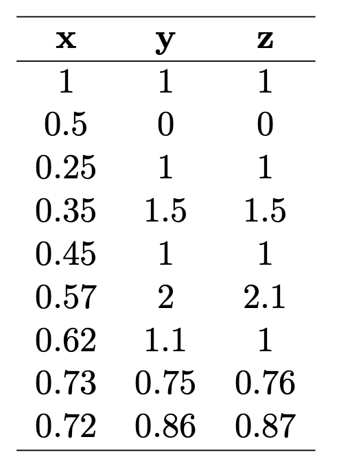
Is \(\mathbf{z}\) adding any new information beyond what is already contained in \(\mathbf{y}\) ?
The two columns have a high covariance (when one increases the other also increases)
Wishlist: The covariance between the columns in the new orthonormal basis should be low - ideally 0
(means that the columns should be linearly independent)
Summary of wishlist
Represent the data using fewer dimensions such that
the data has high variance along these dimensions
the covariance between any two dimensions is low
the basis vectors are orthonormal
Learning Objectives
A quick recap of mean, variance and covariance
What is the covariance matrix?
What is the motivation for PCA?
What is the wishlist for representing data using fewer dimensions?
(achieved)
CS6015: Lecture 20
By Mitesh Khapra
CS6015: Lecture 20
Lecture 20: Principal Component Analysis (the wishlist)


