CS6015: Linear Algebra and Random Processes
Lecture 32: Geometric distribution, Negative Binomial distribution, Hypergeometric distribution, Poisson distribution, Uniform distribution
Learning Objectives
What is the geometric distribution?
What is the hypergeometric distribution?
What is the negative binomial distribution?
What is the Poisson distribution?
What is the multinomial distribution?
How are these distributions related?
Geometric Distribution

\dots \infty~times
The number of tosses until we see the first heads
X:
\mathbb{R}_X = \{1,2,3,4,5, \dots\}
p_X(x) =?
Why would we be interested in such a distribution ?
Geometric Distribution
\dots \infty~times
Hawker selling belts outside a subway station
Why would we be interested in such a distribution ?
Salesman handing pamphlets to passersby
(chance that the first belt will be sold after k trials)
(chance that the k-th person will be the first person to actually read the pamphlet)
A digital marketing agency sending emails
(chance that the k-th person will be the first person to actually read the email)
Useful in any situation involving "waiting times"
independent trials
identical distribution
P(success) = p
Geometric Distribution
\dots \infty~times
Example: k = 5
p_X(5)
F F F F S
P(success) = p
(1-p)
(1-p)
(1-p)
(1-p)
p
\underbrace{~~~~~~~~~~~~~~~~~~~~~~~~~~~~~~~~~~~~~~~~~~~~~~~~~~~}_{(5-1)}
\underbrace{}_{1}
=(1-p)^{(5-1)}p
p_X(k)=(1-p)^{(k-1)}p
Geometric Distribution
\dots \infty~times
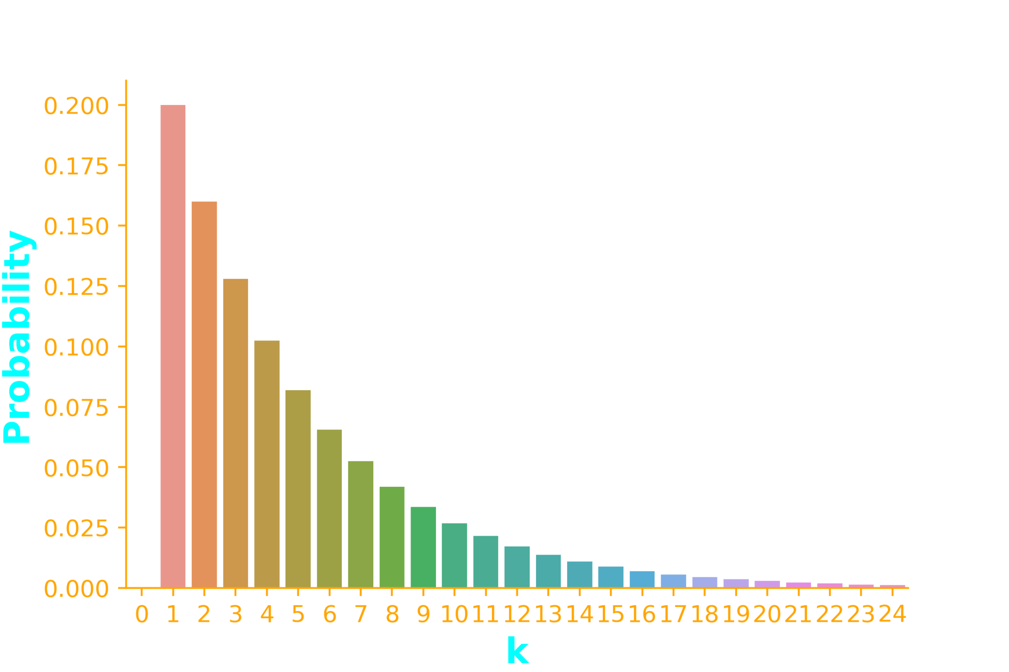
p=0.2
P(success) = p
import seaborn as sb
import numpy as np
from scipy.stats import geom


x = np.arange(0, 25)

p = 0.2
dist = geom(p)
ax = sb.barplot(x=x, y=dist.pmf(x))
Geometric Distribution
\dots \infty~times
p=0.9
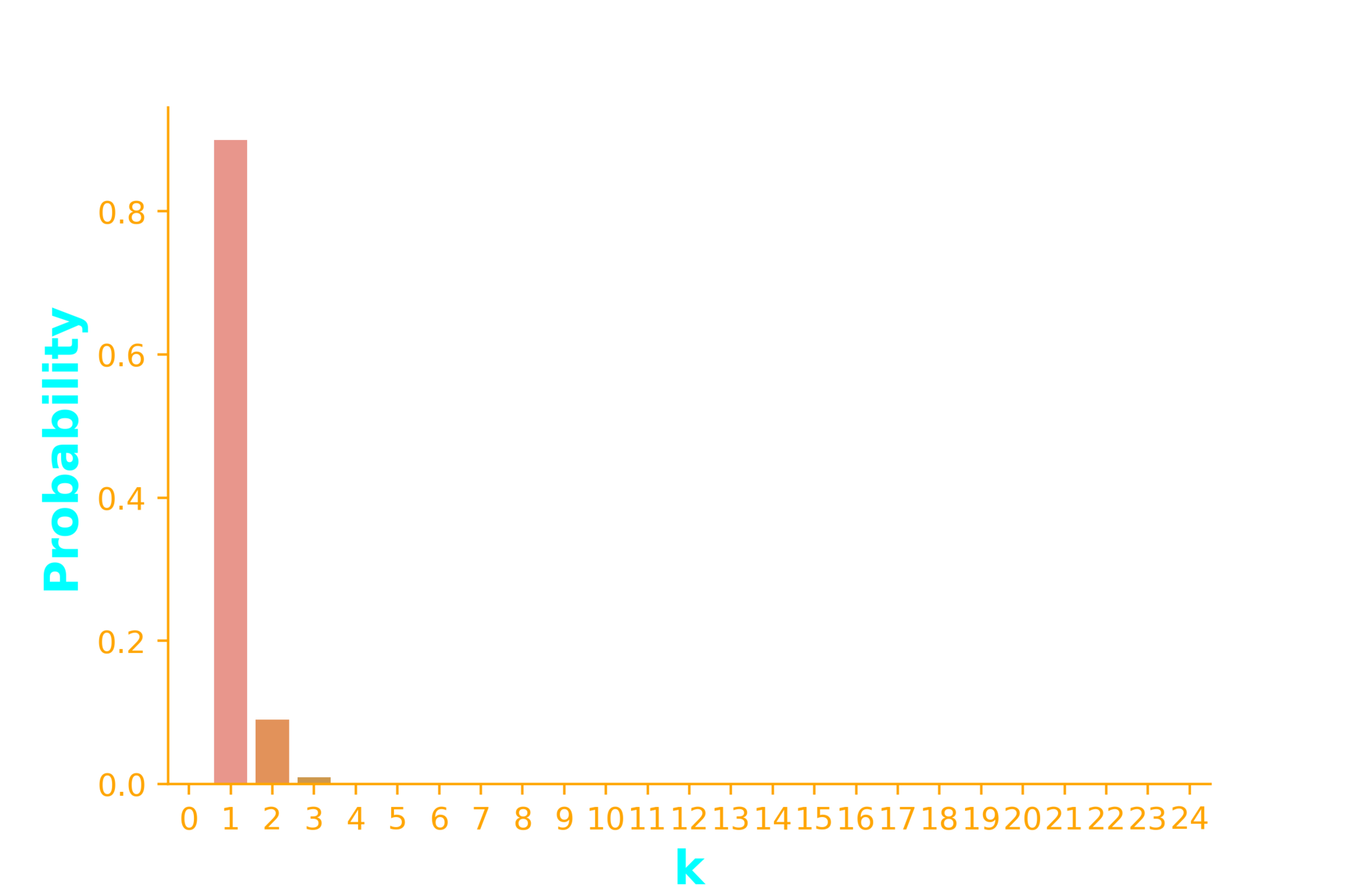
P(success) = p
import seaborn as sb
import numpy as np
from scipy.stats import geom


x = np.arange(0, 25)

p = 0.9
dist = geom(p)
ax = sb.barplot(x=x, y=dist.pmf(x))
Geometric Distribution
\dots \infty~times
P(success) = p
p=0.5
import seaborn as sb
import numpy as np
from scipy.stats import geom


x = np.arange(0, 25)

p = 0.5
dist = geom(p)
ax = sb.barplot(x=x, y=dist.pmf(x))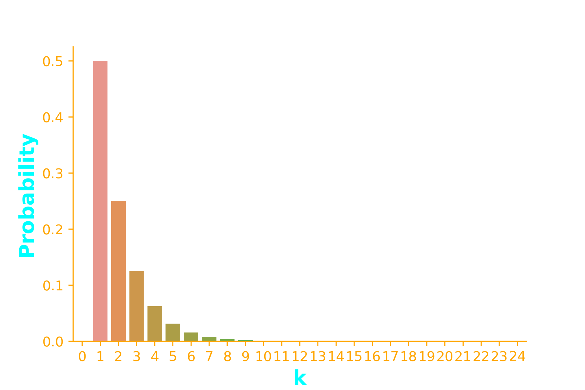
p_X(k)=(1-p)^{(k-1)}p
p_X(k)=(0.5)^{(k-1)}0.5
p_X(k)=(0.5)^{k}
Geometric Distribution
p_X(x) \geq 0
\sum_{k=1}^\infty p_X(i) = 1 ?
Is Geometric distribution a valid distribution?
p_X(k) = (1 - p)^{(k-1)}p
P(success) = p
= (1 - p)^{0}p + (1 - p)^{1}p + (1 - p)^{2}p + \dots
= \sum_{k=0}^\infty (1 - p)^{k}p
= \frac{p}{1 - (1 - p)} = 1
a, ar, ar^2, ar^3, ar^4, \dots
a=p~and~r=1-p < 1
\dots \infty~times
Example: Donor List
A patient needs a certain blood group which only 9% of the population has?
P(success) = p
What is the probability that the 7th volunteer that the doctor contacts will be the first one to have a matching blood group?
What is the probability that at least one of the first 10 volunteers will have a matching blood type ?
\dots \infty~times
Example: Donor List
A patient needs a certain blood group which only 9% of the population has?

p = 0.09
P(X <=10)
p_X(7) = ?
= 1 - P(X > 10)
= 1 - (1-p)^{10}
\dots \infty~times
Negative Binomial Distribution
The number of trials needed to get k successes
X:
\mathbb{R}_X = \{k,k+1,k+2,k+3,k+4, \dots\}
p_X(x) =?
Why would we be interested in such a distribution ?
\dots
A digital marketing agency sending emails
(How many emails should be sent so that there is a high chance that 100 of them would be read?)
independent trials
identical distribution
P(success) = p
Negative Binomial Distribution
An insurance agent must meet his quota of k policies
(How many customers should be approach so that there is a high chance that k of them would buy the policy?)
\dots
Binomial distribution
The number of successes in a fixed number of trials
independent trials
identical distribution
P(success) = p
The difference
Negative Binomial distribution
The number of trials needed to get a fixed number of successes
X
\mathbb{R}_X = \{1,2,3,4,5, \dots, n\}
X
\mathbb{R}_X = \{r,r+1,r+2,r+3,r+4, \dots\}
n
r
\dots
independent trials
identical distribution
P(success) = p
The PMF of neg. binomial
Given
\mathbb{R}_X = \{r,r+1,r+2,r+3,r+4, \dots\}
p_X(x) =?
\# successes = r
Let's find
p_X(i)
for some \(i \in \mathbb{R}_X\)
if \(i\) trials are needed for \(r\) successes then it means that we must have
\(r - 1\) successes in \(i - 1\) trials
and success in the \(i\)-th trial
\dots
independent trials
identical distribution
P(success) = p
Given
\# successes = r
Example, \(r = 3\), \(x=8\)
\underbrace{~~~~~~~~~~~~~~~~~~~~~~~~~~~~~~~~~~~~~~~~~~~~~~~~}_{2~succeses~in~7~trials}
Binomial distribution \(n = 7, p, k = 2 \)
\underbrace{}_{success}
\(p\)
{n\choose k} p^k(1-p)^{n-k}
* p
\dots
The PMF of neg. binomial
S
\dots
independent trials
identical distribution
P(success) = p
Given
\# successes = r
In general, we have \(r \) successes in \(x\) trials
Binomial distribution
\(p\)
{x-1\choose r-1} p^{r-1}(1-p)^{((x-1)-(r-1))}
\(n = x-1, p, k = r-1 \)
* p
The PMF of neg. binomial
S
\underbrace{~~~~~~~~~~~~~~~~~~~~~~~~~~~~~~~~~~~~~~~~~~~~~~~~}_{r-1~succeses~in~x-1~trials}
\underbrace{}_{success}
independent trials
identical distribution
P(success) = p
Given
\# successes = r
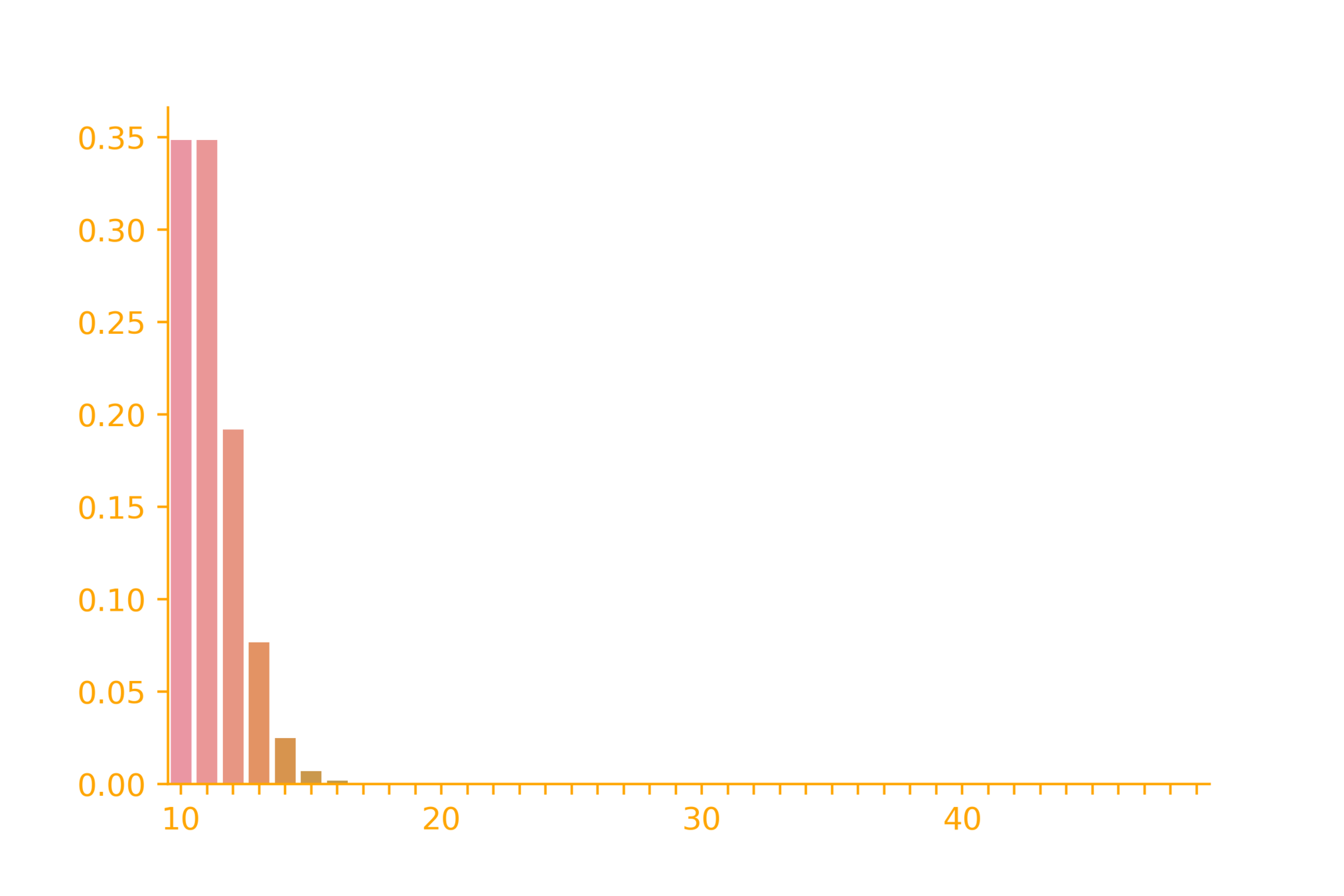
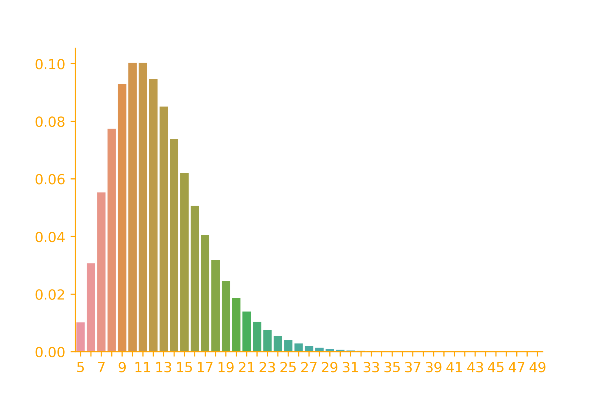
p=0.5
p_X(x) = {x-1\choose r-1} p^{r}(1-p)^{(x-r)}
\dots
The PMF of neg. binomial
r=10
\rightarrow \infty
\dots
independent trials
identical distribution
P(success) = p
Given
\# successes = r
p=0.1
p_X(x) = {x-1\choose r-1} p^{r}(1-p)^{(x-r)}
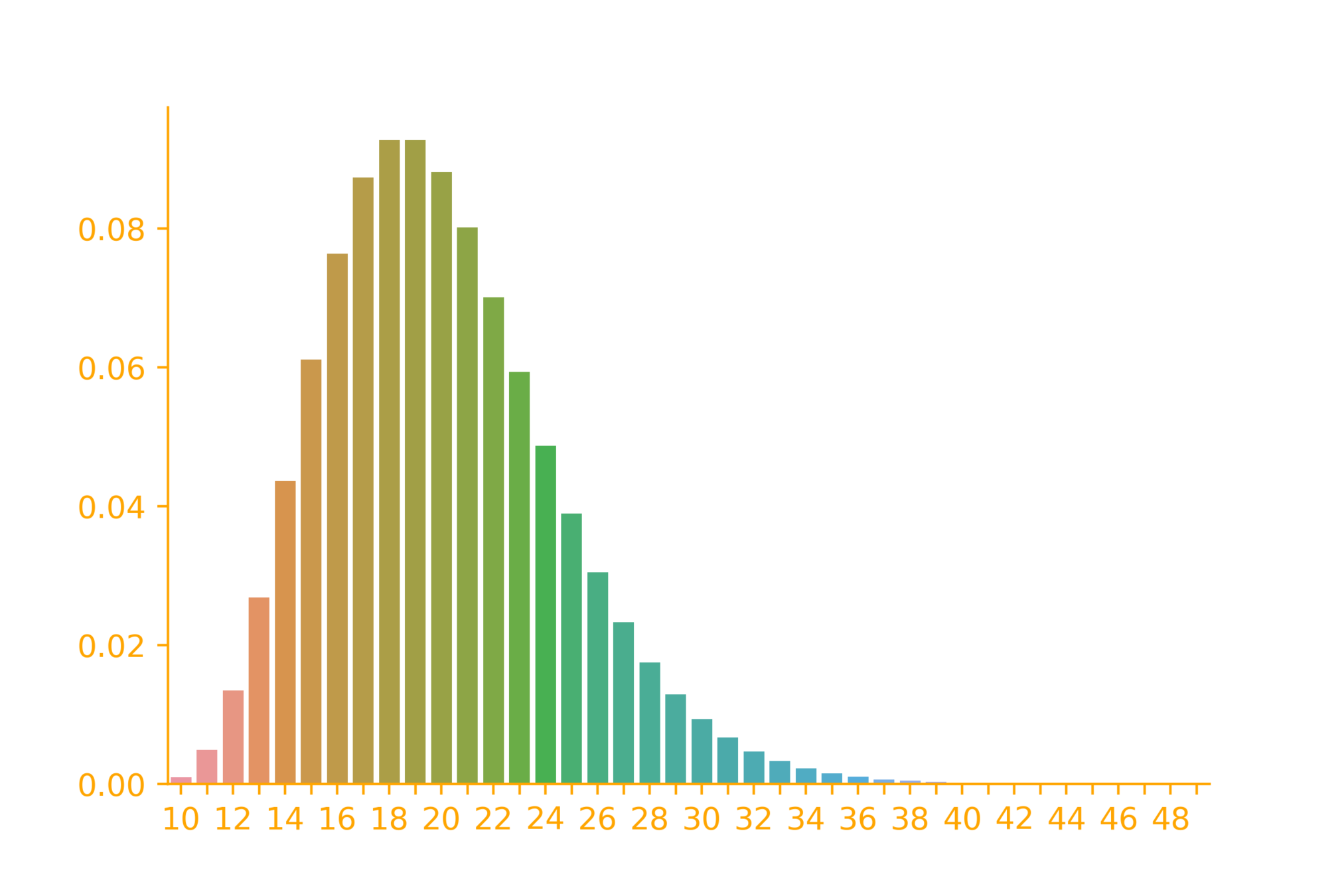
The PMF of neg. binomial
r=10
\rightarrow \infty
\dots \infty~times
independent trials
identical distribution
P(success) = p
Given
\# successes = r
p=0.9
p_X(x) = {x-1\choose r-1} p^{r}(1-p)^{(x-r)}
The PMF of neg. binomial
r=10
\rightarrow \infty
\dots
independent trials
identical distribution
P(success) = 0.4
Example: Selling vadas
Given
\# successes = 5
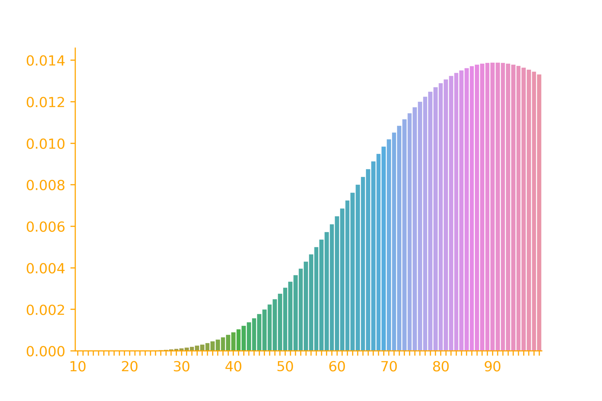
A hawker on a food street has 5 vadas. It is closing time and only the last 30 customers are around. Each one of them may independently buy a vada with a probability 0.4. What is the chance that the hawker will not be able to sell all his vadas?
\overbrace{~~~~~~~~~~~~~~~~~~~~~~~~~~~~~~~~~~~~}^{more~than~30~customers}
very unlikely that the hawker will not be able to sell all the vadas
\dots
independent trials
identical distribution
P(success) = 0.4
Plotting the distribution
Given
\# successes = 5
import seaborn as sb
import numpy as np
from scipy.stats import nbinom
from scipy.special import comb

r = 5
x = np.arange(r, 50)


p = 0.4
y = [comb(i - 1,r - 1)*np.power(p, r)
     *np.power(1-p, i - r) for i in x]

ax = sb.barplot(x=x, y=y)
Hypergeometric Distribution
Randomly sample \(n\) objects without replacement from a source which contains \(a\) successes and \(N - a\) failures
X:
p_X(x) =?
Why would we be interested in such a distribution ?
number of successes
Hypergeometric Distribution
Forming committees: A school has 600 girls and 400 boys. A committee of 5 members is formed. What is the probability that it will contain exactly 4 girls?
trials are not independent
n = 5
a = 600
N-a = 400
committee size
favorable
unfavorable
x = 4
desired # of successes
p_X(4) = \frac{\#~of~committees~which~match~our~criteria}{\#~of~possible~committees}
p_X(4) = \frac{{600 \choose 4} {400 \choose 1}}{{1000 \choose 5}}
= \frac{{a \choose x} {N-a \choose n-x}}{{N \choose n}}
Hypergeometric Distribution
Randomly sample \(n\) objects without replacement from a source which contains \(a\) successes and \(N - a\) failures
X:
\mathbb{R}_X = max(0, n - (N-a)), \dots, min(a, n)
number of successes
p_X(x)= \frac{{a \choose x} {N-a \choose n-x}}{{N \choose n}}
Binomial v/s Hypergeometric
A school has 600 girls and 400 boys. A committee of 5 members is formed. What is the probability that it will contain exactly 4 girls?
trials are dependent
A school has 600 girls and 400 boys. On each of the 5 working days of a week one student is selected at random to lead the school prayer. What is the probability exactly 4 times a girl will lead the prayer in a week?
trials are independent
without replacement
with replacement
p = P(success) = \frac{600}{1000} = 0.6
same on each day
n = 5
k = 4
p_X(k) = {n\choose k} p^{k}(1-p)^{(n-k)}
on first trial
p = P(success) = \frac{600}{1000} = 0.6
on second trial
p = \frac{599}{999}
p = \frac{600}{999}
or
A school has 600 girls and 400 boys. A committee of 5 members is formed. What is the probability that it will contain exactly 4 girls?
p_X^\mathcal{B}(x) = {n\choose x} p^{x}(1-p)^{(n-x)}
p_X^\mathcal{H}(x)= \frac{{a \choose x} {N-a \choose n-x}}{{N \choose n}}
= 0.2591
on first trial
p = P(success) = \frac{600}{1000} = 0.6
on second trial
p = \frac{599}{999}
p = \frac{600}{1000}
or
not very different
= 0.2591
?
Binomial v/s Hypergeometric
When x is a small proportion of N \( ( x \lt\lt N)\), the binomial distribution is a good approximation of the hypergeometric distribution
HW7
on first trial
p = P(success) = \frac{600}{1000} = 0.6
on second trial
p = \frac{599}{999}
p = \frac{600}{1000}
or
not very different
Try this
import seaborn as sb
import numpy as np
from scipy.stats import binom


n=50
p=0.6
x = np.arange(0,n)

rv = binom(n, p)
ax = sb.barplot(x=x, y=rv.pmf(x))
import seaborn as sb
import numpy as np
from scipy.stats import hypergeom
[N, a, n] = [1000, 600, 50] #p = 0.6
x = np.arange(0,n)
rv = hypergeom(N, a, n)
ax = sb.barplot(x=x, y=rv.pmf(x))
From Binomial to Poisson Dist.
Assumptions
arrivals are independent
rate of arrival is same in any time interval
30/day \implies 2.5/ hour \implies (2.5/60)/minute
Suppose you have a website selling some goods. Based on past data you know that on average you make 30 sales per day. What is the probability that you will have 4 sales in the next 1 hour?
From Binomial to Poisson Dist.
Comment: On the face of it, looks like we are interested in number of successes
Question: Can we use the binomial distribution?
Issue: We do not know \(n\) and \(p\), we only know average number of successes per day \(\lambda = 30\)
Suppose you have a website selling some goods. Based on past data you know that on average you make 30 sales per day. What is the probability that you will have 4 sales in the next 1 hour?
From Binomial to Poisson Dist.
Suppose you have a website selling some goods. Based on past data you know that on average you make 30 sales per day. What is the probability that you will have 4 sales in the next 1 hour?
Question: Is there some relation between \(n,p\) and \(\lambda\) ?
If you have \(n\) trials and a probability \(p\) of success then how many successes would you expect?*
* We will do this more formally when we study expectation but for now the intuition is enough
\(np\)
The problem does not mention \(n\) or \(p\)
It only mentions \(\lambda = np\)
This happens in many real world situations
avg. customers/patients per hour in a bank/clinic
avg. ad clicks per day
avg. number of cells which will mutate
From Binomial to Poisson Dist.
Suppose you have a website selling some goods. Based on past data you know that on average you make 30 sales per day. What is the probability that you will have 4 sales in the next 1 hour?
Question: Can we still use a binomial distribution?
\(n = 60 ~minutes\)
\lambda = np
p = \frac{\lambda}{n}
\lambda = 30/day \implies 2.5/ hour \implies (2.5/60)/minute
p = \frac{\lambda}{n} = \frac{2.5}{3600}
Reasoning
\(1~hour = 60 ~minutes\)
each minute = 1 trial
each trial could succeed or fail with \(p = \frac{\lambda}{n}\)
From Binomial to Poisson Dist.
Suppose you have a website selling some goods. Based on past data you know that on average you make 30 sales per day. What is the probability that you will have 4 sales in the next 1 hour?
Question: Is there anything wrong with this argument?
\lambda = np
p = \frac{\lambda}{n}
Reasoning
\(1~hour = 60 ~minutes\)
each minute = 1 trial
each trial could succeed or fail with \(p = \frac{\lambda}{n}\)
Each trial can have only 0 or 1 successes
In practice, there could be 2 sales in 1 min.
Solution: Make the time interval more granular
i.e., increase n
From Binomial to Poisson Dist.
Suppose you have a website selling some goods. Based on past data you know that on average you make 30 sales per day. What is the probability that you will have 4 sales in the next 1 hour?
\lambda = np
p = \frac{\lambda}{n}
Reasoning
\(1~hour = 3600 ~seconds\)
each second = 1 trial
each trial could succeed or fail with \(p = \frac{\lambda}{n}\)
\(n = 3600 ~seconds\)
\lambda = 30/day \implies 2.5/ hour \implies (2.5/3600)/second
p = \frac{\lambda}{n} = \frac{2.5}{21600}
Same issue: There could be 2 sales in 1 sec.
Solution: Make the time interval more granular
i.e., increase n even more
till
\(n \rightarrow \infty\)
From Binomial to Poisson Dist.
Suppose you have a website selling some goods. Based on past data you know that on average you make 30 sales per day. What is the probability that you will have 4 sales in the next 1 hour?
\lambda = np
p = \frac{\lambda}{n}
p_X(k) = \lim {n \choose k} p^k (1-p)^{n-k}
n \to +\infty
(we will compute this limit on the next slide)
p_X(k) = \lim {n \choose k} p^k (1-p)^{n-k}
n \to +\infty
p_X(k) = \lim \frac{n!}{k!(n-k)!} (\frac{\lambda}{n})^k (1-\frac{\lambda}{n})^{n-k}
n \to +\infty
p_X(k) = \lim \frac{n!}{k!(n-k)!} (\frac{\lambda}{n})^k (1-\frac{\lambda}{n})^{n}(1-\frac{\lambda}{n})^{-k}
n \to +\infty
p_X(k) = \lim \frac{n!}{k!(n-k)!n^k} \lambda^k (1-\frac{\lambda}{n})^{n}(1-\frac{\lambda}{n})^{-k}
n \to +\infty
p_X(k) = \lim \frac{n!}{k!(n-k)!n^k} \lambda^k (1-\frac{\lambda}{n})^{n}(1-\frac{\lambda}{n})^{-k}
n \to +\infty
p_X(k) = \frac{\lambda^k}{k!} \lim \frac{n*(n-1)*\dots*(n-k+1)(n-k)!}{(n-k)!n^k} \lim (1-\frac{\lambda}{n})^{n} \lim (1-\frac{\lambda}{n})^{-k}
n \to +\infty
n \to +\infty
n \to +\infty
p_X(k) = \frac{\lambda^k}{k!} \lim \frac{n}{n}*\frac{(n-1)}{n}*\dots*\frac{(n-k+1)}{n} \lim (1-\frac{\lambda}{n})^{n} \lim (1-\frac{\lambda}{n})^{-k}
n \to +\infty
n \to +\infty
n \to +\infty
1
e^{-\lambda}
1
p_X(k) = \frac{\lambda^k}{k!}e^{-\lambda}
Poisson distribution
Poisson Distribution
\(X\): number of events in a given interval of time
or number of events in a given interval of distance, area, volume
\mathbb{R}_X = \{0, 1, 2, 3, \dots\}
events are occurring independently
the rate \(\lambda\) does not differ from one time interval to another
Poisson Distribution (Examples)
number of accidents per hour
number of clicks/visits/sales on a website
For each example convince yourself that in practice
knowing \(n\) and \(p\) is difficult
knowing \(\lambda\) is easy
it makes sense to assume that \(n \rightarrow \infty\) and \(p \rightarrow 0\)
number of arrivals in a clinic, bank, restaurant
number of rats per sq. m. in a building
number of ICU patients in a hospital
number of defective bolts (or any product)
number of people having a rear disease
Poisson Distribution (Examples)
The average number of ICU patients getting admitted daily in a hospital is 4. If the hospital has only 10 ICU beds what is the probability that it will run out of ICU beds tomorrow.
the ICU patients arrive independently
Assumptions:
the arrival rate remains the same in any time interval
the number of admissions follow a Poisson distribution
\(n\) is very large
"success": a patient needs an ICU bed
\(p\) is not known
\(\lambda\) is known
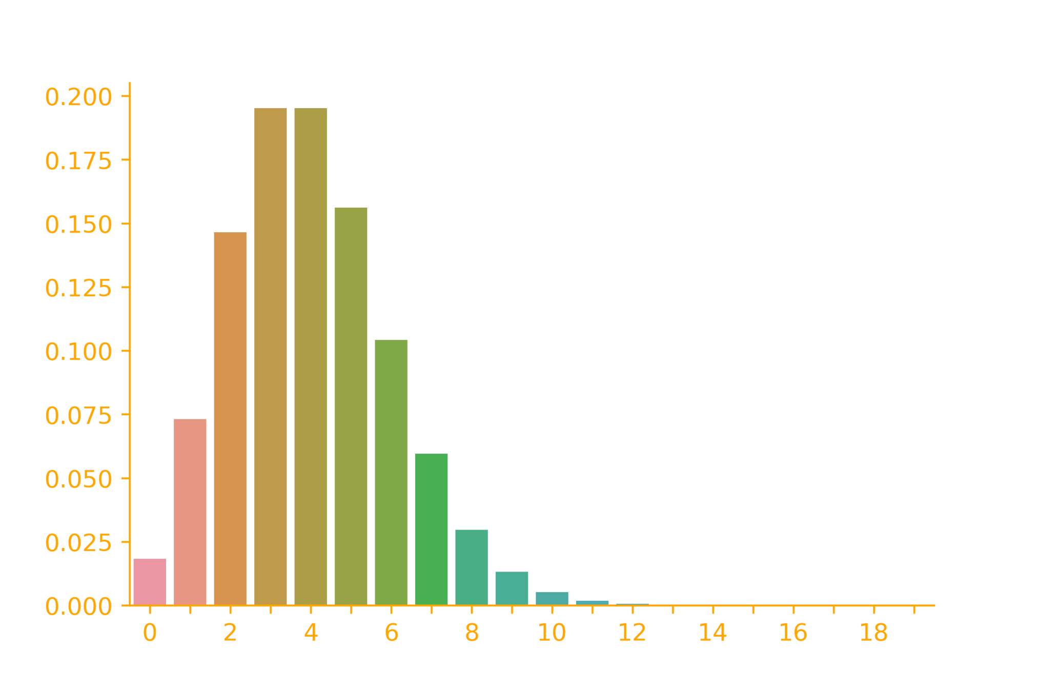
Poisson Distribution (Examples)
p_X(k) = \frac{\lambda^k}{k!}e^{-\lambda}
\lambda = 4
import seaborn as sb
import numpy as np
from scipy.stats import poisson


x = np.arange(0,20)

lambdaa = 4
rv = poisson(lambdaa)
ax = sb.barplot(x=x, y=rv.pmf(x))
\rightarrow \infty
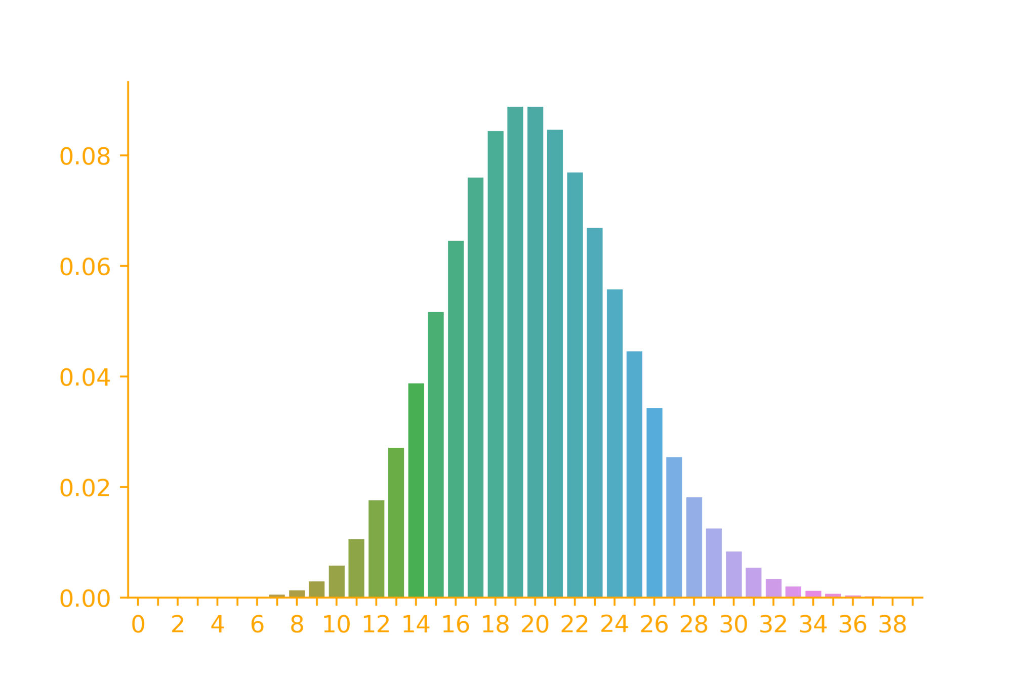
Poisson Distribution (Examples)
p_X(k) = \frac{\lambda^k}{k!}e^{-\lambda}
\lambda = 20
import seaborn as sb
import numpy as np
from scipy.stats import poisson


x = np.arange(0,40)

lambdaa = 20
rv = poisson(lambdaa)
ax = sb.barplot(x=x, y=rv.pmf(x))
\rightarrow \infty
A good approximation for binom.
A factory produces a large number of bolts such that 1 out of 10000 bolts is defective. What is the probability that there will be 2 defective bolts in a random sample of 1000 bolts?
Binomial or Poisson?
X: number of defective bolts
p = 1/10000
n = 1000
p_X^{\mathcal{B}}(2) = {1000 \choose 2} (\frac{1}{10000})^{2}(1 - \frac{1}{10000})^{998}
=0.00452
n is large
p is small
\(\lambda = np = 0.1\)
p_X^{\mathcal{P}}(2) = \frac{(0.1)^2}{2!}e^{-0.1}
=0.00452
Multinomial distribution
Of all the car owners* in India, 50% own a Maruti car, 25% own a Hyundai car, 15% own a Mahindra car and 10% own a Tata car. If you select 10 car owners randomly what is the probability that 5 own a Maruti car, 2 own a Hyundai car, 2 own a Mahindra car and 1 owns a Tata car?
(a generalisation of the binomial distribution)
p_1=0.50
p_2=0.25
p_3=0.15
p_4=0.10
What is/are the random variable(s)?
k_1=5
k_2=2
k_3=2
k_4=1
\Sigma p_i=1
\Sigma k_i=10 = n
X_1= \#~of~Maruti~car~owners
X_2= \#~of~Hyundai~car~owners
X_3= \#~of~Mahindra~car~owners
X_4= \#~of~Tata~car~owners
\mathbb{R}_{X_1}= \{1, 2, ..., 10\}
\mathbb{R}_{X_2}= \{1, 2, ..., 10\}
\mathbb{R}_{X_3}= \{1, 2, ..., 10\}
\mathbb{R}_{X_4}= \{1, 2, ..., 10\}
such~that~X_1+X_2+X_3+X_4 = 10
* this data is not real
Multinomial distribution
Of all the car owners* in India, 50% own a Maruti car, 25% own a Hyundai car, 15% own a Mahindra car and 10% own a Tata car. If you select 10 car owners randomly what is the probability that 5 own a Maruti car, 2 own a Hyundai car, 2 own a Mahindra car and 1 owns a Tata car?
(a generalisation of the binomial distribution)
p_1=0.50
p_2=0.25
p_3=0.15
p_4=0.10
What is the sample space?
k_1=5
k_2=2
k_3=2
k_4=1
\Sigma p_i=1
\Sigma k_i=10 = n
1~~~2~~~3~~4~~~5~~~6~~~7~~8~~~9~~10
all possible selections
4^{10}
What are the outcomes that we care about?
k_1=5
k_2=2
k_3=2
k_4=1
\Sigma k_i=10 = n
* this data is not real
Multinomial distribution
Of all the car owners* in India, 50% own a Maruti car, 25% own a Hyundai car, 15% own a Mahindra car and 10% own a Tata car. If you select 10 car owners randomly what is the probability that 5 own a Maruti car, 2 own a Hyundai car, 2 own a Mahindra car and 1 owns a Tata car?
(a generalisation of the binomial distribution)
p_1=0.50
p_2=0.25
p_3=0.15
p_4=0.10
How many such outcomes exist?
* this data is not real
What is the probability of each such outcome?
k_1=5
k_2=2
k_3=2
k_4=1
\Sigma p_i=1
\Sigma k_i=10 = n
1~~~2~~~3~~4~~~5~~~6~~~7~~8~~~9~~~10
{10 \choose 5}
{10-5 \choose 2}
{10-5-2 \choose 2}
{10-5-2-2 \choose 1}
\frac{10!}{5!(10-5)!}
\frac{(10-5)!}{2!(10-5-2)!}
\frac{(10-5-2)!}{2!(10-5-2-2)!}
\frac{(10-5-2-2)!}{1!(10-5-2-2-1)!}
\frac{10!}{5!2!2!1!}
= \frac{n!}{k_1!k_2!k_3!k_4!}
\frac{n!}{k_1!k_2!k_3!k_4!}
p_1^{k_1}p_2^{k_2}p_3^{k_3}p_4^{k_4}
Multinomial distribution
Of all the car owners* in India, 50% own a Maruti car, 25% own a Hyundai car, 15% own a Mahindra car and 10% own a Tata car. If you select 10 car owners randomly what is the probability that 5 own a Maruti car, 2 own a Hyundai car, 2 own a Mahindra car and 1 owns a Tata car?
(a generalisation of the binomial distribution)
p_1=0.50
p_2=0.25
p_3=0.15
p_4=0.10
* this data is not real
k_1=5
k_2=2
k_3=2
k_4=1
\Sigma p_i=1
\Sigma k_i=10 = n
1~~~2~~~3~~4~~~5~~~6~~~7~~8~~~9~~~10
p_{X_1,X_2,X_3,X_4}(x_1,x_2,x_3,x_4) =
\frac{n!}{k_1!k_2!k_3!k_4!}p_1^{k_1}p_2^{k_2}p_3^{k_3}p_4^{k_4}
Relation to Binomial distribution
Of all the car owners* in India, 50% own a Maruti car, 25% own a Hyundai car, 15% own a Mahindra car and 10% own a Tata car. If you select 10 car owners randomly what is the probability that 5 own a Maruti car, 2 own a Hyundai car, 2 own a Mahindra car and 1 owns a Tata car?
(a generalisation of the binomial distribution)
p_1=0.50
p_2=0.25
p_3=0.15
p_4=0.10
* this data is not real
k_1=5
k_2=2
k_3=2
k_4=1
\Sigma p_i=1
\Sigma k_i=10 = n
1~~~2~~~3~~4~~~5~~~6~~~7~~8~~~9~~~10
p_{X_1,X_2,X_3,X_4}(x_1,x_2,x_3,x_4) = \frac{n!}{k_1!k_2!k_3!k_4!}p_1^{k_1}p_2^{k_2}p_3^{k_3}p_4^{k_3}
Of all the car owners* in India, 70% own a Maruti car, and 30% own other cars. If you select 10 car owners randomly what is the prob. that 6 own a Maruti ?
p_1=p=0.7
p_2= 1- p = 0.3
k_1=6
k_2=n -k
\Sigma p_i=1
\Sigma k_i= n
p_{X_1,X_2}(x_1,x_2) = \frac{n!}{k!(n-k)!}p^{k}(1-p)^{n-k}
(binomial distribution)
Relation to other distributions
with replacement
without replacement
\(2\) categories
\(n(>2)\) categories
Binomial
Hypergeometric
Multinomial
Multivariate Hypergeometric
Bernoulli
\(X\)
number of successes in a single trial
\(\mathbb{R}_X\)
\(p_X(x)\)
Binomial
number of successes in \(n\) trials
Geometric
number of trials to get the first success
Negative binomial
number of trials to get the first \(r\) successes
Hypergeometric
number of successes in n trials when sampling without replacement
Poisson
\(n\) is large, \(p\) is small or \(n,p\) are not known, \(np = \lambda\) is known
Multinomial
number of successes of each type in \(n\) trials
\(0, 1\)
\(0, 1, 2, \dots, n \)
\(1, 2, 3, \dots, \)
\(r, r+1, r+2, \dots, \)
\(max(0, n - (N-a))\), \( \dots, min(a, n) \)
\(0, 1, 2, \dots, \)
\(p^x(1-p)^{1-x}\)
\({n \choose x}p^x(1-p)^{n-x}\)
\frac{{a \choose x} {N-a \choose n-x}}{{N \choose n}}
\frac{\lambda^x}{x!}e^{-\lambda}
\frac{n!}{x_1!x_2!...x_r!}p_1^{x_1}p_2^{x_2}...p_r^{x_r}
\((1-p)^{x-1}p\)
{x-1\choose r-1} p^{r}(1-p)^{(x-r)}
\(E[X]\) \(Var(X)\)
Uniform Distribution
Experiments with equally likely outcomes
X:
p_X(x) = \frac{1}{6}~~~\forall x \in \{1,2,3,4,5,6\}
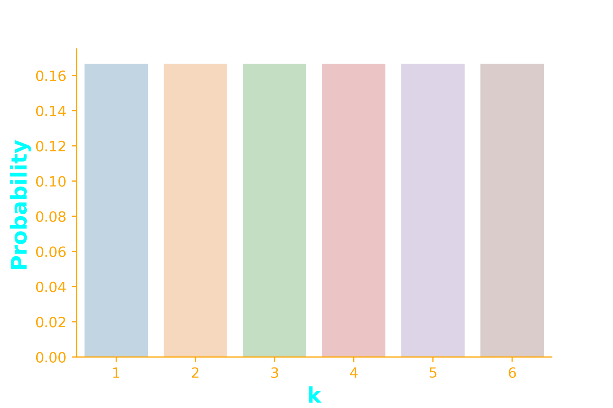
outcome of a die
Uniform Distribution
Experiments with equally likely outcomes
X:
p_X(x) = \begin{cases} \frac{1}{b - a + 1}~~~a \leq x \leq b \\~\\ 0~~~~~~~~~otherwise \end{cases}
outcome of a bingo/housie draw
p_X(x) = \frac{1}{100}~~~1 \leq x \leq 100
\mathbb{R}_X = \{x: a \leq x \leq b\}
Uniform Distribution
Special cases
p_X(x) = \begin{cases} \frac{1}{b - a + 1} = \frac{1}{n}~~~1 \leq x \leq n \\~\\ 0~~~~~~~~~otherwise \end{cases}
a = 1 ~~~~ b = n
p_X(x) = \begin{cases} \frac{1}{b - a + 1} = 1~~~x = c \\~\\ 0~~~~~~~~~otherwise \end{cases}
a = 1 ~~~~ b = c
Uniform Distribution
p_X(x) \geq 0
\sum_{k=1}^\infty p_X(i) = 1 ?
Is Uniform distribution a valid distribution?
p_X(x) = \frac{1}{b - a + 1}
=\sum_{i=a}^b \frac{1}{b-a+1}
=(b-a+1) * \frac{1}{b-a+1} = 1
Puzzle
If you have access to a program which uniformly generates a random number between 0 and 1 (\(X \sim U(0,1)\)), how will you use it to simulate a 6 sided dice?
Learning Objectives
What is the geometric distribution?
What is the hypergeometric distribution?
What is the negative binomial distribution?
What is the Poisson distribution?
What is the multinomial distribution?
How are these distributions related?
(achieved)
CS6015: Lecture 32
By Mitesh Khapra
CS6015: Lecture 32
Lecture 32: Geometric distribution, Negative Binomial distribution, Hypergeometric distribution, Poisson distribution, Uniform distribution


